Blog

Stochastic consolidation of lifelong memory | Scientific Reports – Nature.com

Thank you for visiting nature.com. You are using a browser version with limited support for CSS. To obtain the best experience, we recommend you use a more up to date browser (or turn off compatibility mode in Internet Explorer). In the meantime, to ensure continued support, we are displaying the site without styles and JavaScript.
Advertisement
Scientific Reports volume 12, Article number: 13107 (2022)
378 Accesses
1 Altmetric
Metrics details
Humans have the remarkable ability to continually store new memories, while maintaining old memories for a lifetime. How the brain avoids catastrophic forgetting of memories due to interference between encoded memories is an open problem in computational neuroscience. Here we present a model for continual learning in a recurrent neural network combining Hebbian learning, synaptic decay and a novel memory consolidation mechanism: memories undergo stochastic rehearsals with rates proportional to the memory’s basin of attraction, causing self-amplified consolidation. This mechanism gives rise to memory lifetimes that extend much longer than the synaptic decay time, and retrieval probability of memories that gracefully decays with their age. The number of retrievable memories is proportional to a power of the number of neurons. Perturbations to the circuit model cause temporally-graded retrograde and anterograde deficits, mimicking observed memory impairments following neurological trauma.
Understanding the principles governing long-term memory is a major challenge in theoretical neuroscience. The brain is capable of storing information for the lifetime of the animal, while continually learning new information, so the brain must face the stability—plasticity dilemma: keep changing in order to learn new memories, but do so without erasing existing information. In humans, forgetting curves (retrieval probability vs. age of memory, sometimes referred to as retention curves), are found experimentally to be gracefully decaying with memory age, allowing for non-zero probability of retrieval for memories tens of years of age1,2,3,4. While retrieval probability curves monotonically decrease with memory age, the lifetime of individual memories is more intricate, and seemingly stochastic—we might not be able to retrieve a memory from last week, but can retrieve a much older one. Thus, the retrieval of memories does not depend on the memories’ age alone.
Early attractor neural network models of long-term memory suffer from catastrophic forgetting: when the number of encoded memories is lower than a critical value, memories are retrievable with high precision, but when it is above that critical value, none of the memories can be retrieved5,6,7. Incorporating synaptic decay into the circuit enables continual learning, such that at any point in time recent memories are stable. However, the predicted forgetting curves exhibit a critical memory age, all memories newer than some age are almost perfectly retrievable, while all older ones are destroyed (a palimpsestic behavior-old information is deleted in favor of new information)8,9,10,11,12,13. This is in contrast to the gracefully decaying forgetting curves in humans. Furthermore, the critical age is of the order of synaptic decay time, hence memories older than this time cannot be retrieved. Another class of memory models which avoid catastrophic forgetting are models with bounded (continuous or discrete) synaptic strengths14,15. These models also give rise to a palimpsestic behavior qualitatively similar to synaptic decay models: only new memories up until a critical age are retrievable, while the older memories are not.
One of the main methods of studying the mechanisms of human memory is through memory disorders. Amnesic patients show a variety of patterns of forgetting. One is anterograde amnesia-reduced memory retrieval of events encoded after the onset of the disturbance to the circuit, presumably due to the inability to encode or store new memories. Another pattern is temporally-graded retrograde amnesia—when the probability of retrieval of memories encoded a short time before the pathology onset is lower than that of older events, giving rise to non-monotonic forgetting curves (an effect also known as Ribot’s law). Retrograde amnesia is typically explained by invoking memory consolidation theory, suggesting that memories must go through a stabilization process that is disrupted by the proximal onset of the disturbance16,17,18,19,20,21,22.
In addition to possible cellular mechanisms, memory consolidation at the system level is mediated through a rehearsal process—reactivating memories in wakefulness or during sleep23,24,25,26,27. Several computational models have been proposed for memory consolidation through rehearsals28,29,30,31,32,33,34,35,36. However, all reported results were confined to a small number of memories; none demonstrated memory functionality and forgetting curves in a large circuit with a number of retrievable memories scaling with the number of neurons. None of the models obtain the scaling of capacity and memory lifetime with the number of neurons and other intrinsic parameters.
Here we present a neural network model for lifelong continual learning and memory consolidation. Our model continuously stores patterns of activity by Hebbian learning, and combines synaptic decay with stochastic nonlinear reactivation of memories. Our model generates intricate and rich memory forgetting behavior. Retrieval probability curves decay smoothly with memory age (exponentially or even as a power law), with characteristic times that can be orders of magnitude longer than the synaptic decay time. In addition, due to the stochasticity of the consolidation process, there is a large variability in the survival of individual memories of the same age. We show that at any given time, the number of retrievable memories scales as a power of the number of neurons, exhibiting adequate memory functionality expected for a robust neuronal circuit with distributed memories. The power approaches unity for high rehearsal rate and the capacity approaches linear behavior with the number of neurons.
Perturbations of the model circuit give rise to complex patterns of memory deficits, temporally-graded retrograde and anterograde amnesia, the details of which depend on the size as well as the nature of the perturbation. Our theory relates global measures of memory functionality (memory capacity, characteristic memory lifetime) to intrinsic cellular and circuit parameters, such as synaptic decay rate and reactivation statistics, and provides new insight into how the brain builds and maintains the body of memories available for retrieval at each point in an animal’s life.
We model the lifelong memory acquisition and forgetting processes using a recurrent neural network, continuously experiencing Hebbian learning of new activity patterns (”memories”). Following initial memorization, memories are strengthened by stochastic rehearsal events, each increasing the Hebbian contribution of the rehearsed memory to the network synaptic connectivity matrix (‘the memory efficacy’), thereby enhancing their retrievability. In addition, the synapses spontaneously degrade with time, mimicking the well-known synaptic turnover in biological neural networks. For simplicity, our model consists of a single neuronal population, and every synapse is allowed to be positive or negative. The retrieval of a memory at a certain moment in time is determined by both its current efficacy as well as its random interference with other stored memories. The rate of rehearsals of a given memory is self-consistently determined by its retrievability, such that a more easily retrievable memory will be revisited more frequently than a less retrievable one, and a memory that loses its retrievability will not be rehearsed anymore. In this framework, memories begin their life with a fixed initial efficacy, which is subsequently increased by each rehearsal, and decays between rehearsals. As long as a memory is revisited frequently enough, its amplitude will be larger than the threshold efficacy required for retrieval. However, due to the stochastic nature of the rehearsals process, there will be a period of time eventually when the time lag between two rehearsals will be too long, such that the efficacy of the memory will drop too low, making the memory irretrievable, and therefore forgotten. The age at which a certain memory will be forgotten is therefore stochastic and may range from the order of the synaptic decay timescale to several orders of magnitude longer. In the following sections we give a detailed description of our memory model, present its properties and explain how these properties emerge from our model’s dynamics.
Our model is based on the sparse version of the Hopfield attractor network model of associative memory5,6. Memories are sparse7,37,38,39,40,41, uncorrelated N-dimensional binary activation patterns (N is the number of neurons) and are stored as fixed points of a recurrent neural network dynamics with binary neurons. We assume that the neural activation threshold is adjusted dynamically so that the population activity level maintains the same sparsity as the memories (see “Methods”, in “The effects of structural perturbations on memory function” this assumption is modified). Synaptic dynamics are governed by three processes: Deterministic exponential synaptic decay8,11 (first term in Eq. (1)), Hebbian learning42 of new memories (second term in Eq. (1)), and Hebbian consolidation of old memories following their reactivation (third term in Eq. (1)),
Here (J_{ij}(t)) is the strength of the synapse between neurons i and j at time t (symmetric in i and j), (xi _i^l) is the i-th element of the memory introduced first at time (t=l) and it is given by:
Here f is the fraction of neurons active in a memory state (the sparseness level). According to the above equation, new memories enter in each time interval (Delta t) and synapses decay at a rate (1/tau), representing the finite lifetime of synapses43. The last term represents a Hebbian strengthening of old memories following a sequence of reactivation events that occur for memory k at times denoted by (t_{k}) (which will be specified below). The factor b denotes the size of synaptic modification due to a single consolidation event of an old memory, assumed to be smaller than the Hebbian amplitude of learning a new memory (i.e. (b< 1)). The resulting connectivity matrix can be written as:
(A_l(t)) is the efficacy of memory l at time t. The ability to recall a memory depends on the level of noise, which originates from random interference with other memories. Its variance is proportional to the sum of the squares of all efficacies (see “Methods”):
We define the critical efficacy (A_c), as the efficacy for which a memory pattern loses its stability. (A_c) is proportional to the interference noise (Delta), with the proportionality constant depending only on the sparseness:
Due to the reduction of overlap between memories, The critical efficacy is increased when f is decreased. The factor a(f) can be approximated by (see Supplementary Information (SI) section 1):
This approximation holds for the f regime we consider throughout this study. For (f=0.01) (which we will use throughout the paper), (a approx 4.7).
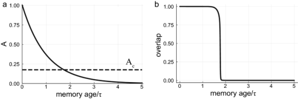
Without rehearsals, our model is similar to previous models of associative memory with forgetting8,10,11, in which memory efficacies decay exponentially with age, (A_l(t)=exp (-(t-l)/tau )) (Fig. 1a). Using Eq. (4), the interference noise equals (Delta ^2approx f tau /(2N)). For (tau >tau _0), where (tau _0=2N/(f a^2(f))) (see Eq. (5)), (A_c) increases above unity (the initial efficacy) and no memory will be retrievable. This global catastrophic forgetting is similar to the behavior of the Hopfield model after reaching memory capacity, where the interference effect is too strong and all memory states lose their stability5,6. If (tau < tau _{0}), recent memories are retrievable, while memories older than a critical age (t_0 = frac{tau }{2} log left( frac{tau _0}{tau } right)) are forgotten (Fig. 1b). Thus, for short decay times, this model allows for continual learning of recent memories without global catastrophic forgetting. However, it predicts an unrealistic age-dependent catastrophic forgetting, where all memories up to a critical age are almost perfectly retrievable, and all older memories are completely forgotten. This sharp transition happens despite the graceful exponential decay of efficacies with age, and results from the collective effects of memory stability in the network.
In what follows we will show that when stochastic rehearsals are taken into account, the behavior changes dramatically, generating more realistic memory forgetting trajectories and allowing for lifelong memories.
(a) Pure forgetting. A memory efficacy trajectory as a function of time (solid line). The critical efficacy (A_c) is plotted as a dashed line. (b) Overlap of the network state with a memory state as a function of the memory age. The overlap is a measure of memory retrievability—after initializing the network near a memory state, the overlap of the nearby attractor network activity will be close to unity for retrievable memories and small compared to one for irretrievable memories. Here (N=8000), (f=0.01), (tau =2240). The catastrophic age here is (sim 1.73tau), resulting in a capacity (number of retrievable memories) of  0.5N. Note the very large value of (tau) needed to support this capacity—this will be addressed in later sections.
To specify the statistics of reactivations, we revert to the continuous time version of Eq. (1) which yields the efficacies dynamics:
With (A_{l}(t)=0) for (t<l) and (A_{l}(l)=1). The reactivations are modeled as a point process
where (t_l) are the times at which memory l was rehearsed. To specify the rate of the reactivation process, we hypothesize that this process is more likely to yield a Hebbian strengthening of memories with a large basin of attraction. The rationale is that during reactivation periods, the system is more likely to visit memories with large basins of attraction and stay there for a significant period of time triggering their Hebbian strengthening . In particular, memories that at some point in time lost their stability and are not attractors of the dynamics (i.e., have vanishing basin of attraction) will not be reactivated, will experience fast pure decay, and will be forgotten. Hence we model reactivation events as inhomogeneous Poisson processes, with mean rate (r_l (t)equiv langle R_l(t) rangle) , which is proportional to the memory’s basin of attraction size:
where (lambda) denotes the maximal reactivation rate. As in Eqs. (4) and (5), at all times (A_c(t)=a(f) cdot Delta (t)) . The nonlinear function F denotes the size of the basin of a memory and depends on the ratio of the memory efficacy over the critical capacity (A_c) (Fig. 2a). We derive the function F by numerical calculation of memories’ basin of attraction size for different values of (A/A_c) (see “Methods” section and SI for details). At any given time, only memories with non-zero basin size (i.e., (A_l(t)>A_c rightarrow F>0)) are retrievable and might be reactivated. Note that since the interference (Delta (t)) depends on the efficacies of all memories (Eq. (4)), the reactivation rates of all memories are coupled in Eq.  (9) via (A_c).
It is useful to first consider the average dynamics, replacing the reactivation point process by its mean rate, Eq. (9). For a given (A_c), the resulting self-consistent equation for the steady state efficacies,
possesses two stable fixed points: one at zero and another one when the two competing processes, decay and reactivation, balance each other ((A_{text {fp}}), Fig 2a). Due to the rapid saturation of the function F, for most of the parameter regime (A_{text {fp}}sim blambda tau).
To fully understand the system’s behavior we need to consider the dynamics of (A_c) itself as well as the stochastic nature of the process. Initially, when the first memories enter the system, (A_cpropto Delta) is very small and the memory efficacies consolidate around the value (A_{text {fp}}sim blambda tau). As more memories are encoded, the interference grows and so does the critical efficacy (red line in Fig. 2b). When the critical efficacy is large enough, fluctuations in reactivation times lead some memory efficacies to drop below (A_c), making these memories irretrievable. A steady state is achieved when the flux of memories arriving at the system and consolidated is balanced by the rate of memories forgetting due to the drop of their efficacy below (A_c). At this stage, (A_c) reaches a fixed equilibrium value and so does the mean number of retrievable memories. The specific identity of the retrievable memories varies with time—some are forgotten while new ones are being consolidated. The distribution of efficacies at equilibrium (Fig. 2c) consists of two modes: The first is the contribution of the forgotten memories, below (A_c), which diverges at small A as (p(A)=tau / A). The second, above (A_c), is a mode around (A_{text {fp}}) representing the retrievable memories.
(A_c) increases as the amplitude b and number of reactivations per decay timescale (lambda tau) increase, due to increased interference (Fig. 2d). For moderate reactivation strength, (A_c) is well below both the encoding strength (A(0)=1) and the consolidation fixed point as seen in the examples in Fig. 2b,c. As reactivation strength grows, (A_c) increases and approaches 1, affecting adversely the consolidation process, as will be seen in the next section.
Stochastic memory dynamics. (a) Blue: basin of attraction size F as a function of memory efficacy A. Orange dashed: (A/tau), the negative of the deterministic decay term in Eq. (7). Importantly, F is zero for (A<A_c). Here (lambda tau =5), (A_c=0.4). (b) Example memory efficacies vs. age of the system. Memories enter with efficacy (A(0)=1), rehearsal efficacy (b=0.3). Most of them increase towards (A_{fp}approx blambda tau approx 1.5), and fluctuate around it. Large enough fluctuations can take efficacies below (A_c) (e.g, cyan curve at (age/tau approx 40), yellow curve at (age/tau approx 120)). Some memories are alive for a very short time (e.g., green curve) and some for very long (e.g., red, blue curves). (c) Distribution of memory efficacies after saturation of (A_c). (d) Equilibrium values of (A_c) as a function of (blambda tau) for different (lambda tau) values. Here (tau =160,; N=8000).
Importantly, in our model, the time of forgetting of memories at a given age is highly variable, ranging from a fraction of the decay time (tau) (for unfortunate memories that weren’t rehearsed fast enough after learning), and up to hundreds of (tau) for well-rehearsed memories (Fig. 2b). Nevertheless, on average, memory retrievability decreases with memory age, and this is captured by the forgetting curve—the probability of retrieving a memory as a function of its age, after a steady state has been reached (Fig. 3a,b). This curve exhibits an exponential tail with a long time constant, denoted as the consolidation time (tau _c)—a direct result of the long time required for a large fluctuation in reactivation rates to form such that consolidated efficacies decrease from around (A_{text {fp}}) to (A_c) (SI). The consolidation time enhancement factor (tau _c / tau) can reach several orders of magnitude, allowing memories to survive for very long times compared to the intrinsic timescales of the system (as shown in Fig. 3c,d). For fixed consolidation parameters (lambda tau) and b, consolidation time normalized by (tau) decreases with (tau) due to increased interference (Fig. 3d).
For fixed (tau), consolidation time increases sharply with (lambda tau) and b (Fig. 3c). However, increasing these parameters may adversely affect the consolidation process. When (blambda tau) is of order 1, most of the memories experience consolidation, as is the case in Fig. 3a . However when (blambda tau gg 1), (A_c) is close to the encoding efficacy (Fig. 2d). This causes a significant number of memories not to get consolidated. Therefore, the forgetting curve exhibits an initial fast decay with a characteristic time (tau), in addition to the slow decay time (tau _c) (Fig. 3b). To quantify this effect, we measure the consolidation probability of memories, (p_c), defined as the chance of a memory efficacy to reach (A_{fp}), and therefore become part of long-lived memories. (p_c) decreases as a function of the reactivation strength from (p_c=1), for (blambda tau <1), to zero for strong reactivation (Fig. 3d). The consolidation probability (p_c) together with (tau _c) are the key consolidation parameters.
(a, b) The forgetting curve. The probability of retrieval as a function of memory age. Blue dots: full network simulation results (see “Methods”). Red solid lines: results of a mean field approximation (“Methods”). An exponential fit with characteristic decay time (approx 18tau) is shown in green (dash-dot line) in (a), and a double exponential fit with characteristic decay times (approx tau) and (approx 38tau) in (b). The retrieval probability for pure forgetting is shown in black (dashed line). In (a) (N=8000), (tau =160), (lambda tau =5), (b=0.3). In (b) same parameters as (a) except (b=0.25,; lambda tau =10). (c) Blue (left y axis): Consolidation probability vs. (blambda tau) for different (lambda tau) values. Green (right y axis): Consolidation time (tau _c) normalized by synaptic decay time (tau) vs. (b lambda tau) for different (lambda tau) values. Here (tau =160). (d) Consolidation time (tau _c) normalized by synaptic decay time (tau) vs. (tau) for different (lambda tau) values. Blue curve: (lambda tau =5, b=0.3). Green curve: (lambda tau =10,b=0.25).
We define the network’s memory capacity as the number of memories retrievable (memories with (A>A_c)) in the equilibrium phase after long encoding time (Fig. 4). The capacity can be evaluated as the area under the forgetting curve. Hence, it can be approximated as ((1-p_c)tau +p_ctau _c), where (p_ctau _c) is the contribution from consolidated memories and fraction of memories that are consolidated and the first term is the contribution from unconsolidated memories. As seen previously, (tau _c) increases with (blambda tau), while (p_c) decreases with (blambda tau)—less memories are consolidated, but the consolidated ones live longer. Maximal capacity is achieved when (b lambda tau approx A(0)=1), which is the maximal value that allows for (100%) of the memories to get consolidated.
To assess the efficiency of information storage in the network it is important to evaluate the dependence of the capacity on the network size, N. In previous ’pure forgetting’ models8,10 the synaptic decay time was assumed to scale linearly with N, resulting in memory capacity (t_0) which is proportional to N. The same holds for our model. However, this scaling results in extremely large, biologically implausible, synaptic decay times for large networks. Here we assume that (tau) is a property of individual synapses and is independent of network size. Under this condition, the capacity in the pure forgetting model increases only logarithmically with N, Fig. 4c.
Interestingly, we find that in our model, the capacity scales as a power law of the number of neurons, with a power that approaches unity for large (lambda tau) values (Fig. 4c,d). To approximate the power analytically (for the parameter range where (p_c approx 1)), we first approximate (A_c), assuming that the main contribution to the interference noise comes from consolidated, retrievable memories (SI, sec.3):
Now, under the assumption that (p_c approx 1) and that the mean rehearsal rate is (~lambda tau), we get (SI):
Figure 4c,d show the approximation gives a reasonable fit to the dependence of the capacity on N. Note the significant increase in capacity compared to the pure forgetting model.
Memory capacity. (a) The number of retrievable memories divided by N as a function of (b lambda tau) for different average number of rehearsals per characteristic decay time ((lambda tau)) values. The dashed line shows the capacity of the pure forgetting model. Here (N=8000,; tau =160). (b) The number of retrievable memories divided by N as a function of (tau) for different (lambda tau) values. (c) Capacity vs. N (logarithmic, base 10), solid lines show simulation results, dashed lines are analytical approximation. Here (tau =160,; b=0.3). (d) The power of N vs. (lambda tau) (black), and the analytical approximation (red). Here (tau =160,; b=0.3).
So far we have assumed that all memories are encoded initially by Hebbian plasticity with the same amplitude (A(0)=1) (eq. 1). In reality, memories might differ in their encoding strength, for instance, due to factors such as attention, or emotional context. Thus, it is important to explore the effect of a distribution of initial encoding strengths. As long as most of the initial efficacies are in the neighborhood of (blambda tau), the global memory properties such as (A_c), forgetting curve, and capacity are not affected drastically. However, individual memories with initial efficacy below (A_c) are forgotten, while memories with A(0) larger than (blambda tau) have slightly enhanced consolidation properties, as is confirmed in Fig. 5a for an exponential distribution of A(0) with mean 1.
To better elucidate the effect of inhomogeneity in A(0), we consider in Fig. 5b,c the case of a Bernoulli distribution, (A(0) in {1, a_0}) with equal probability. For small (a_0) compared to (blambda tau =1.5), the consolidation probability for memories with (A(0)=a_0) decreases drastically and vanishes for (a_0) below (A_c approx 0.39) (Fig. 5b). When (a_0) increases above 1, consolidation probability of these memories increases until it reaches 1 for (a_0 approx b lambda tau). On the other hand, memories with (A(0) =1) are only moderately affected by changing (a_0). The mean lifetime of memories with (A(0)=a_0 < 1) drops considerably (Fig. 5a,c). This is, however, due to averaging the lifetime of all memories including those that did not consolidate. Importantly, in our model, memories with small (a_0) that did reach the neighborhood of the fixed point have the same long lifetime as other consolidated memories, independent of the original encoding strengths as shown by the dashed lines in Fig. 5c. Note that inhomogeneous initial efficacy distribution alone will not give rise to memories with lifetime much larger than the synaptic decay time scale, due to the exponential decay—for a lifetime of 10 times the decay time scale, the initial efficacy will have to be (text {exp}(10)) times larger than the critical efficacy. In any initial efficacy distribution, such a memory will be extremely rare, because the critical efficacy is proportional to the square root of the distribution’s second moment.
Initial condition distribution. (a) Here A(0) for each memory is drawn from an exponential distribution with unity mean. Blue points are values for single memories, and the red line shows the mean. Note that the spread in lifetimes at each encoding strength is a result of the stochastic rehearsal process, which yields an exponential distribution of lifetimes and is present also in the uniform A(0) case. (b) Consolidation probability vs. (a_0), which is the initial efficacy of half of the memories (the others have (A(0)=1)). Values for memories introduced with (A(0)=1) are shown in blue, and for memories introduced with (A(0)=a_0) are shown in red. (c) Memory mean lifetime (time from insertion to forgetting) as a function of (a_0). Same scenario and coloring as in (a). Dashed lines are averaged lifetimes of consolidated memories only. Parameters: (N=8000,; f=0.01,; lambda tau =5,; b=0.3)
In this section we analyze the effect of damage to the circuit on memory storage and retrieval. In previous sections, we assumed for simplicity that the neuronal firing threshold is automatically adjusted to guarantee a fixed mean activation level, f (see “Methods”). Here we assume that the firing threshold is fixed since we anticipate that part of the effect of perturbation is the disruption of the level of activity. Importantly, in the case of constant threshold, the dependence of (A_c) on (Delta) is not linear. It has a non-zero value for small (Delta) reflecting the requirement for the encoding efficacy to be large enough for neurons to cross the threshold. Above some critical (Delta), (A_c) rises abruptly, causing all memories to lose stability, due to over-activation of the network when the noise level is high (Fig. S4). At equilibrium (Delta) is below but close to the critical value (for the presented parameter range). In this scenario, the properties of the unperturbed system are similar to those of the fixed activity scenario, with a memory capacity that depends on the threshold value. For the presented results we used the threshold value 0.36 which maximizes capacity in unperturbed conditions (See SI).
We first consider perturbations of the synaptic learning and consolidation processes by adding white noise (chi) to the synaptic dynamics, for all (tge t_{text {onset}}),with a diffusion coefficient D,
The effect of this noise is approximately an additive contribution to the total variance of local fields
After the noise onset, (Delta) increases rapidly above its critical value, causing a sharp increase in (A_c), and the blocking of rehearsals for all memories. This in turn causes a rapid decrease in magnitude of stored memory efficacies, leading to a decrease in (Delta) below the critical value and a decrease in (A_c) to a value which is between the value before the onset and the value just after the noise onset. This new equilibrium value of (A_c), with reduced capacity, occurs over (sim tau) (Fig. 6a). Although overall reduction in capacity may be mild for moderate D values, there is a large reduction in the retrieval probability of memories that were encoded around the perturbation onset time, due to the sharp transient increase in (A_c). In contrast, memories that have already been consolidated suffer only a mild reduction in survival probability (relative to unperturbed memories of the same age). Likewise, newly entered memories have a high probability of consolidation, since they experience the equilibrium value of (A_c) and their retrieval probability is similar to the unperturbed case (Fig. 6b).
Another perturbation we consider is the death of a fraction of the synapses. We model the effect of the synaptic death by multiplying the connectivity matrix (J_{ij}) by a binary random dilution ({0,1}) matrix:
Unlike the additive noise considered above, synaptic dilution process is multiplicative, reducing both the effective efficacy of each memory (by a factor (1-p)), and the interference noise (Delta) (by factor (sqrt{1-p})), and in general reduces the signal to noise ratio (“Methods”). After the dilution onset, (A_c) barely changes (due to the weak dependence of (A_c) on (Delta) in the constant threshold scenario), while all the efficacies are reduced, causing a reduction of retrievability that spreads over the entire age range ( Fig. 6c,d) and a new equilibrium is achieved slowly. Interestingly, neural adaptation (modeled here as a decrease in the neural activation threshold) can reduce the memory loss due to silencing (also reported in44,45,46), by reducing the minimum efficacy required for activation, i.e., (A_c), thereby recovering some of the gap between memory efficacies and (A_c) (Fig. 7). Thus, our model predicts a qualitative difference in the effects of the two types of perturbations: synaptic dilution affects memories of all ages, causing a reduction in capacity that develops over a long time and can be partially compensated for by threshold adaptation, while additive synaptic noise results in a deficit largely confined to the time of the perturbation onset, and fast convergence to a new equilibrium.
Perturbations and memory deficits. (a) The ratio between the capacity with and without injected noise vs. the diffusion coefficient D. (b) Retrieval probability vs. memory age with noisy synaptic dynamics ((D=6)). Noise onset was before: (5tau) (green), (10tau) (blue), (20tau) (purple), (40tau) (brown). The control (black) is simulated with noiseless dynamics. (c) The ratio between the capacity with and without synaptic dilution vs. the silenced synapses fraction p. (d) Retrieval probability vs. memory age for random synaptic dilution ((p=0.1)). Coloring as in (b). (e) Same as (c), but with (p=0.2). Memories of all ages are affected, with some non-monotonicity caused by the small efficacies of newly learned memories, dropping more easily below (A_c). (f) Combination of synaptic dilution and noisy synaptic dynamics, (D=6) and (p=0.1). Coloring as in (b). Parameters: (N=8000,; tau =160,; lambda tau =10,; b=0.25)
Effect of threshold adaptation. Blue bars show capacity with threshold optimized for the noiseless case ((theta _0=0.36)). Green bar shows capacity with threshold optimized for low dilution (p=0.1, (theta _1=0.31)). Red bar shows capacity for threshold optimized for high dilution (p=0.2, (theta _2=0.29)). Parameters: (N=8000,; tau =160,; lambda tau =10,; b=0.25)
Experiments showing that the time scale of synaptic and spine turnover is variable43, and observations of power law memory retention curves in some memory studies1,2,3,4,47 encourage consideration of the properties of synaptic dynamics with heterogeneous decay time constants, yielding,
where the efficacies (A_{l}^{ij}(t)) contributed by each synapse obey
The mean efficacy of each memory is the average over these contributions,
where (langle ..rangle _{tau _{ij}}) denotes the average over the distribution of synaptic time constants. Likewise, the noise term is proportional to the sum of second moments of the efficacies:
As an example, we show the case where the decay time constants are power law (Pareto) distributed , i.e., (P(tau )propto tau ^{-(alpha +1)} ; ; tau ge tau _0,alpha >0) (“Methods”). In the absence of rehearsals (pure decay), there will be a global catastrophic forgetting for (alpha le 1), where the mean of the decay rate, and therefore the interference noise, diverges. For (alpha >1) there will be a catastrophic age dependent forgetting, as in the case with a uniform decay time scale (See13 SI). With stochastic nonlinear rehearsals, for large (alpha) the forgetting curve is approximately exponential, similar to the single (tau) case (Fig. 8b). This is because the dominant contribution comes from the shortest time (tau _0). Interestingly, for intermediate values ((1<alpha <1.8)), the forgetting curves have an approximately power-law decay (Fig. 8a). In this regime, the retrieval probability is affected by contributions from a broad range of time constants: neither the minimal (tau) nor outliers with very large values are dominant.
Power-law synaptic decay characteristic time distribution. (a) Retrieval probability as a function of memory age on log-log scale (blue), with power-law fit in black (dashed line, slope(approx 1)). Here (lambda tau =5) for the empirical mean (tau), (b=0.25), the power (alpha =1.5). The minimal (tau) is 20. (b) Goodness of fit ((R^2)) for the forgetting curve using an exponential function (orange, dash-dot) and power-law function (blue), as a function of the power parameter of the characteristic time distribution.
We have proposed a stochastic self-amplified memory consolidation mechanism and showed that it leads to smooth forgetting curves that extend much longer than the synaptic decay time. Our model provides estimates for the global long-term memory properties such as the capacity of the network, the shape of the forgetting curve and the average lifetime of memories. Translating synaptic decay time to realistic times is hard. In rodents, spine turnover time is estimated to be of the order of several weeks in the hippocampus and up to a year in the cortex43,48,49,50,51. In humans, these times may be longer given the lower metabolic rate52,53; however, there are no direct experimental evidence. In addition, the model synaptic decay time (tau) is in units of the mean inverse rate of encoding of episodic memories, which is hard to estimate, but it is likely to be of the order of weeks. Thus, assuming a human spine turnover time of the order of months yields (tau) of the order of tens of months, which could lead to mean memory lifetime of several years. At present, these estimates are speculative.
We have considered two types of perturbations to the memory circuit: synaptic death and increased synaptic noise. Both types of damage result in reduced retrievability of memories introduced prior to the damage onset, a phenomenon known in the literature as retrograde amnesia16,17,18,19. Due to the consolidation effect in our model, the amnesia is temporally graded: memories learned just before the noise onset are more severely affected than older ones, because they didn’t have enough time to consolidate, and were more fragile at the onset time. This effect is more prominent in the case of increased synaptic noise than synaptic dilution, due to the sharper drop in basins of attraction size after the noise addition. Perturbations cause a drop in retrieval performance of new memories entering after the perturbation onset, a manifestation of anterograde amnesia. This effect is temporally graded as well, being more severe for memories introduced just after the onset, and is especially prominent deficit in the additive noise case. Another interesting difference is the approach to a new equilibrium, which is fast in the case of additive noise but slow in the dilution. In addition, threshold adaptation can compensate part of the memory dysfunction caused by dilution, but not by additive noise.
Our model also allows for exploration of transient perturbations (SI), where the damage lasts for a finite time window54. In this case there is again a temporally-graded retrograde amnesia. Interestingly, new memories introduced after the end of the event not only regain retrievability, but can even improve their retrievability compared to control. This is due to the increased forgetting rate during the event, which results in lower interference noise and increased rehearsal rate after the event end.
The predictions of our model should be contrasted with the pure decay model where similar perturbations reduce the capacity (maximal age for retrievable memories), but don’t introduce any non-monotonicity in the forgetting curve, which is still a step function, but with a reduced width.
In the classical theory of systems memory consolidation16,17,18,20, the interaction between the hippocampus (HC) and the cortex plays a central role, with HC storing memories for short periods of time, and following rehearsals, memories are transmitted to the cortex for long-term storage. In the recent Multiple Trace Theory (MTT)20,29 autobiographic memories are stored for long term memory in both HC and cortex and consolidated through rehearsals that establish multiple memory traces in HC. This model shares some key elements with our theory, such as ongoing, life-long consolidation of memories and rehearsals which make memories more robust to perturbations. However, it is unclear how MMT can scale to large numbers of stored memories. In addition, in29 the rehearsal statistics (new trace formation) don’t depend on the robustness of the memories, nor does the model take into account interference between memories.
In the pseudo-rehearsal model28, new memories are learned in batches. After each batch is learned, there is a series of presudo-rehearsals, which are learning of fixed point states that are found by random initialization of the network’s state. This model implements stochastic rehearsals explicitly, and it reduces loss of old information by the pseudo-rehearsals. While in our model we use Hebbian, one-shot learning of new memories, the pseudo-rehearsal model relies on multi step gradient descent of each memory batch, which is generally a less biologically plausible learning algorithm. In addition, the authors present results only for a single, small size network and it is not clear how the results scale with the size of the network, nor how the increase of memory life time depends on the different properties of the model.
A few studies used neural network models where rehearsals are modeled as random visits of learned memories31,33,36, or implicit rehearsals (via memory traces embedded in the noise correlations30). In33 the authors shows the effects of rehearsals on a large number of learned memories. Yet they do not explicitly model the ”Hippocampus” part of the model where rehearsals occur, and they do not provide quantitative relations between the model’s performance and the different parameters, such as number of neurons in the ”neocortex” part. In30,31,36 The authors study the effect of rehearsals in networks with specific size, small number of memories, that don’t scale with the network size. It is not clear how their results scale with the network size, and how does the enhancement in memory lifetime depends on the different network properties. The authors of30,36 consider rehearsals of a finite batch of previously encoded memories rather than with life-long learning as in our study. Benna and Fusi13 studied memory storage with complex synapses, where a consolidation process is implemented in the dynamics of synapses, with a cascade of synaptic characteristic times. They show that their mechanism gives rise to a power-law decay of the signal-to-noise ratio (SNR, equivalent to (A_l(t)/Delta (t)) in our model) with age. However, this model still exhibits a deterministic catastrophic age-dependent forgetting, such that all memories older than a critical age are non-retrievable, whereas all newer memories are almost perfectly retrievable. A recent phenomenological model47 derives a power-law form for memory retention curves with a power of 1 or smaller. A power close to 1 for intermediate ages is consistent with our result for a power law distribution of synaptic decay time. However, at present, it is unclear whether the experimental paradigms and time scales in which a power law is observed are relevant to life long episodic memory.
Fiebig and Lansner35 proposed a three component model, each with different synaptic decay rate, which performs continual learning with self-generated rehearsals. Similar to our work, they study the effects of perturbations and show similarities to human data. However, this work does not provide an analysis of the model, and does not explore the dependence on the different parameters such as network size and synaptic decay time and rehearsal rates. Comparison with our results is hampered also by the fact that synaptic decay in their model is an active process, dependent on memory arrivals among other factors. In general, none of the past models provide quantitative analysis of the memory capacity and the memory lifetime statistics, while enabling lifelong learning and avoiding global and critical-age catastrophic forgetting.
There is a fundamental difference between the catastrophic forgetting nature in long term memory network models, which we address here, and what is called catastrophic forgetting in machine learning, and deep learning especially55,56,57. In the deep learning literature, it is assumed that if all the data was available all the time the model was able to learn from it and successfully solve the relevant task. In other words, the model is in a regime below its capacity limits, and the problem is the online, incremental presentation of the data, which causes stability-plasticity issues. In contrast, when modeling long term memory we assume that there is too much information to be stored- even if the data to be stored was available all the time and learning wasn’t online, still we would encounter catastrophic forgetting due to crossing of the model capacity limit.
In this paper we don’t explicitly model the rehearsals process—how the system moves between activation states and visits different attractors. Possible mechanisms could be destabilization of attractors by adaptation36,58 or transitions induced by random initialization processes31. These mechanisms will generate a rate of rehearsals per memory that depends on its basin of attraction size, as in our model, but whether the rate is simply proportional to the basin’s size as we assume is yet to be tested.
Our model can be extended in a variety of ways, including more biologically plausible neuronal and synaptic integration. For example, detailed neuron models with rich morphologies and dendritic structure might influence the memory capacity and lifetime, in addition to the number of neurons. In addition, our model does not obey Dale’s law, and restricting neurons to be either excitatory or inhibitory, while also allowing different long term and short term plasticity dynamics for the different populations, will likely introduce richer memory properties.
Studying more synaptic decay characteristic time distributions, such as bimodal distributions where one synapse population decays much slower than another population, could also give rise to interesting memory properties. A relevant example is an inhibitory population with slow synaptic decay, interacting with an excitatory population with faster synaptic decay. We limit ourselves in this work to the mechanism of synaptic decay, while other mechanisms, such as bounded, discrete synapses14,15 can also prevent global catastrophic forgetting. Due to the qualitative similarity of the behavior of such models to synaptic decay models (palimpsestic behavior with critical age catastrophic forgetting), we expect that this model will respond similarly to the introduction of stochastic rehearsals. Additionally, our framework allows for analyzing the effect of other types of perturbations, such as post-traumatic stress disorder amnesia59,60.
The stochastic nonlinear rehearsal mechanism proposed in our work is, to the best of our knowledge, the first large-scale memory model that gives rise to realistic gracefully decaying forgetting probability curves, with exponential or power law tails depending on synaptic decay rate distribution. Our model’s capacity scales as a power law of the number of neurons, with a power that approaches unity for a large mean number of rehearsal events per synaptic decay time. Our model’s capacity interpolates between two extreme cases—for low rehearsal rate it approaches the pure forgetting case (logarithmic scaling of the capacity with the number of neurons), where learning is incremental and synapses decay, and for high rehearsal rate it approaches linear scaling of capacity with N, as in the static case without synaptic decay, where memories are stored (not necessarily incremental, they can be available forever) until capacity is reached and then all memories become irretrievable. Our model predicts that the onset of perturbation to the circuit, in the form of synaptic noise, leads to non-monotonic memory deficits affecting more strongly memories encoded around perturbation onset time, which have not yet a chance to consolidate. The richness of the model behavior in normal and diseased conditions provides a theoretical framework for predictions and testing against empirical data on human memory.
As described in section II, memories are modeled as sparse, uncorrelated N dimensional activation patterns (N is the number of neurons), and the synaptic dynamics are governed by three processes: deterministic synaptic decay with rate (1/tau), Hebbian learning of new memories, and rehearsal of old memories, which is the central novelty of our model. In continuous time, Eq. (1) becomes:
The rehearsals are modeled as a point process
Inserting the ansatz (3), we get that (A_{l}) obeys the differential equation:
With (A_{l}(t)=0) for (t<l) and (A_{l}(l)=1).
The single neuron dynamics are binary, and given by:
where (sigma _(t)) is the state of neuron i at time t, (Theta (x)) is the Heaviside step function, (h_i(t)) is the local field (total input received by neuron i at time t):
and (theta) is a threshold, set at every time step such that the total activation of the network is maintained and equal to fN. This can be thought of as the effect of an inhibitory population, regulating the total population activity (practically, in full simulations, at each time step we choose the fN neurons with the largest local fields and set their state to one, and all the others are set to zero).
We would like to find the relation between memory stability, measured by the memory pattern’s basin of attraction size, and the efficacy of the memory and all other memories in the system. First, we define two useful quantities: (f_{+}^{l}) is the probability of a neuron to be active in the current state given that it is active in the memory pattern (xi ^{l}). (f_{-}^{l}) is the probability of a neuron to be active in the current state given that it is not active in the memory pattern (xi ^{l}). In other words, (f_{+}^{l}) is the fraction out of the neurons active in memory state l that are active in the current state. (f_{-}^{l}) is the fraction out of the neurons not active in memory state l that are active in the current state. We will omit the l dependence of (f_{pm }) from now on. In terms of these quantities,
For clarity, in this section instead of the memory patterns definition we use above (Eq. (2)) we define the patterns in an equivalent, more explicit way:
, and we normalize the connectivity matrix accordingly.
The overlap between memory pattern l and the system’s state (sigma)
Now, assume that the current state is close to the memory state (xi ^{l}). The input to neuron i which is active in memory pattern l ((xi _{i}^{l}=1)):
Averaging (h_{i}^{+}) over memories realizations gives (A_l(1-f)M_{l}), and the variance:
Now, because the system state is close to the memory state (xi ^{l}), we can assume it is uncorrelated with all other memory states. Hence, there are contributions only from terms with (j=j’,;n=n’):
Applying the central limit theorem, we approximate (h_{i}^{+}) by a Gaussian variable with mean (A_l(1-f)M_{l}) and variance (Delta ^2). Now, (f_{+}) is the probability for (h_{i}^{+}) to be larger than (theta), which is given by the complimentary error function, (H(x)=frac{1}{sqrt{2pi }}int _{x}^{infty }text {exp}(-0.5t^{2})dt):
In a similar way (same noise term, mean equals (-A_lM_{l}f)) we find for (f_{-}) (for (fll 1)) :
Note that we didn’t set the threshold (theta), but instead demanded a constant population activation f. Equations (25), (27), (31) and (32) allow us to write an equation for the overlap dynamics:
where
and
Therefore, the equation for the overlap fixed points is:
Now, we numerically find the fixed points for M at a given (A/Delta) by running the dynamics described by Eq. (33). Typically (for large enough (A/Delta)), there will be a stable fixed point at (M=0), a stable fixed point (0<M_s le 1) and an unstable fixed point (0<M_{us}<M_s). We approximate the basin of attraction size as the distance (M_s-M_{us}). This way, we obtain the basin size as a function of (A/Delta), (F(A/Delta )). We check the validity of our approximations by simulating a full neural network model and checking numerically the basin of attraction sizes, and find good agreement (SI), which is the basis for the good agreement in retention curves between the mean field simulations and the full network simulation (Fig. 3a,b) . We define the critical efficacy (A_c) as the efficacy for which (M_s=M_{us}) (meaning, the non-zero overlap solution loses stability). This happens approximately when (M_s=M_{us} approx 0.85). As one can see from Eq. (36), the fixed points depends only on the ratio (A/Delta) and on f, and therefore (A_c/Delta) is only a function of f, and we can write (A_c=a(f) Delta). For (f=0.01) (the typical value we use throughout the manuscript) we find numerically that (a(f)approx 4.7) . Analytical approximation for a(f) is given in the SI.
In our simulations, we first numerically solve the coupled stochastic differential equations for the efficacies (Eq. (7)). Theoretically our model considers infinite number of memories. However, practically we solve the equations for a finite but large number of memory efficacies, typically (200tau – 1000tau), chosen such that (A_c) saturates to its steady state value. We measure time in units of the lag between the introduction of two consecutive memories (assumed constant). At every integration time step dt (small compared to all characteristic timescales of the system, typically (dt=0.05/lambda)), a rehearsal event might occur for each memory with (A_lge A_c). We generate a uniform random number between 0 and 1 and compare it to (lambda cdot F(A_l(t)/Delta (t) cdot dt). A rehearsal event of memory l will happen at time t if the uniform random number is smaller than (lambda cdot F(A_l(t)/Delta (t) cdot dt). This approximates the statistics of a non-homogeneous Poisson process. By averaging over many such realizations (typically 500), we calculate the efficacy histogram, capacity (counting how many efficacies are above (A_c)) and retrieval probabilities (by checking the probability for the efficacy of a memory introduced l time units into the past to be retrievable now). These calculations are referred to as ”mean field simulations”, and they don’t include generation of random memories and building the connectivity matrix.
When simulating the full network model, after generating the efficacies, we randomly generate memory patterns (binary vectors of dimension N) to be stored, and build the connectivity matrix according to Eq. (3). Then, to measure retrievability, we initialize the network’s state at a memory pattern, and let the binary neurons dynamics run until they settle to a steady state. Then, we measure the overlap between the pattern and the steady-state activity. We say a memory is retrievable if the overlap is (ge 0.85). For measuring the basin of attraction sizes of the memory patterns, we generate an initial state by randomly flipping the state of units in the memory pattern (conserving the total activation fN), and run the dynamics until convergence. Then we measure the overlap between the final state and the memory pattern. We keep increasing the number of flipped units until the final state has an overlap smaller than (ge 0.85) with the memory state. We define the normalized basin size as the maximal number of flips allowing for a large overlap divided by 2fN, the maximal number of flips. Results are shown in the SI.
The synaptic dynamics in the presence of Gaussian noise is presented in Eq. (13). It is straightforward to show that a solution to the equation can be written as:
with (A_{l}(t)) obeying Eq. (7) as before. The nonlinear effect of the noise arises through the self consistent requirement, that the rehearsal rate of memory l is proportional to the basin of attraction size of this memory, which depends on (A_l) and on (Delta). We calculate (Delta) with the injected noise (Eq. (14)) the same way we calculated (Delta) without noise above. Here there is a non trivial mixed term involving the average (langle A_l(t) chi _{ij}(t) rangle), which we found numerically to be negligible for the parameter range we are interested in.
The random silencing is done by multiplying the connectivity matrix (J_{ij}) by a binary matrix:
We would like to calculate the effect of the dilution on the memory efficacies dynamics, and for that we need to find the effect on (A_l(t)) and on (Delta (t)). Let us calculate the local field near memory l as before:
Taking the mean over memories and over (C_{ij}) realizations (denoted by []) we get:
Here 〈 〉 denotes average over memories realizations. As one can see, the efficacies are scaled by a factor of (1-p). We assumed here we can neglect correlations between (A_l) and (C_{ij}). The second moment:
There are two contributions arising from the (C_{ij}) randomness. Now, when calculating the local field variance, the term proportional to ((1-p)^2) is exactly canceled by the squared mean, and we are left with:
where (tilde{Delta }^2) is the local field variance without dilution.
Now, we obtain the efficacies modified dynamics by using these expressions for the signal and noise to calculate the basins of attraction sizes as before.
Assuming synapse (J_{ij}) has a decay rate (epsilon _{ij}), and all memories have unit initial efficacy. Memory l appears for the first time at time l. The learning dynamics is:
In continuous time,
Assuming all synapses starts at zero value, the solution can be written as:
Let us define efficacies
(A_{l}^{ij}) obeys the differential equation:
With (A_{l}^{ij}(t)=0) for (t<l) and (A_{l}^{ij}(l)=1).
Given that the decay rates have a probability density (rho (epsilon )), let us define:
and
Including normalization and sparseness considerations,
Now let us calculate the mean local field on neuron i in a state near memory state k, and assume (xi _{i}^{k}=1):
Taking an average over the memories realizations and the decay rates, we get:
And the variance:
The second term does not include summation over all memories, and therefore it is negligible for large N values (the first term is O(1) while the second is (O(N^{-2})). This leads to Eq. (19).
For each synapse we generated synaptic decay characteristic times from a power law (Pareto) distribution with density:
In this distribution, for (alpha <1) the mean diverges. We scaled the resulting (tau _0^{ij}) values by a uniform factor: (tau ^{ij}=2omega cdot N cdot tau _0^{ij}). We fixed (omega) value for the average number of rehearsals per mean decay time (R_0), and used it to set the (lambda) parameter by dividing (R_0) by the empirical average of the generated decay times. Next we solved the stochastic differential Eq. (48) numerically. The rehearsals are generated with time dependent rates proportional to the basin of attraction size, now as a function of the average and variance of the memory efficacies over all synaptic timescales.
All presented results were obtained by a custom code written in the Julia language. Code will be made available upon request. No experimental data was used or generated.
Rubin, D. C. On the retention function for autobiographical memory. J. Verbal Learn. Verbal Behav. 21, 21–38 (1982).
Article  Google Scholar 
Rubin, D. C. & Schulkind, M. D. The distribution of autobiographical memories across the lifespan. Mem. Cogn. 25, 859–866. https://doi.org/10.3758/BF03211330 (1997).
CAS  Article  Google Scholar 
Meeter, M., Murre, J. M. & Janssen, S. M. Remembering the news: Modeling retention data from a study with 14,000 participants. Mem. Cogn. 33, 793–810 (2005).
CAS  Article  Google Scholar 
Averell, L. & Heathcote, A. The form of the forgetting curve and the fate of memories. J. Math. Psychol. 55, 25–35 (2011).
MathSciNet  MATH  Article  Google Scholar 
Hopfield, J. J. Neural networks and physical systems with emergent collective computational abilities. Proc. Natl. Acad. Sci. 79, 2554–2558 (1982).
ADS  MathSciNet  CAS  PubMed  PubMed Central  MATH  Article  Google Scholar 
Amit, D. J., Gutfreund, H. & Sompolinsky, H. Storing infinite numbers of patterns in a spin-glass model of neural networks. Phys. Rev. Lett. 55, 1530 (1985).
ADS  CAS  PubMed  Article  Google Scholar 
Amit, D. J., Gutfreund, H. & Sompolinsky, H. Information storage in neural networks with low levels of activity. Phys. Rev. A 35, 2293 (1987).
ADS  MathSciNet  CAS  Article  Google Scholar 
Nadal, J., Toulouse, G., Mézard, M., Changeux, J. & Dehaene, S. Neural networks: Learning and forgetting. In Computer Simulations and Brain Science (Cambridge University Press, 1986).
Google Scholar 
Parisi, G. A memory which forgets. J. Phys. A: Math. Gen. 19, L617 (1986).
ADS  Article  Google Scholar 
Mézard, M., Nadal, J. & Toulouse, G. Solvable models of working memories. J. Phys. 47, 1457–1462 (1986).
MathSciNet  Article  Google Scholar 
Akaho, S. Capacity and error correction ability of sparsely encoded associative memory with forgetting process. In International Conference on Artificial Neural Networks, 707–710 (Springer, 1993).
Storkey, A. J. & Valabregue, R. The basins of attraction of a new hopfield learning rule. Neural Netw. 12, 869–876 (1999).
PubMed  Article  Google Scholar 
Benna, M. K. & Fusi, S. Computational principles of synaptic memory consolidation. Nat. Neurosci. 19, 1697–1706 (2016).
CAS  PubMed  Article  Google Scholar 
Tsodyks, M. Associative memory in neural networks with binary synapses. Mod. Phys. Lett. B 4, 713–716 (1990).
ADS  MathSciNet  Article  Google Scholar 
Amit, D. J. & Fusi, S. Learning in neural networks with material synapses. Neural Comput. 6, 957–982 (1994).
Article  Google Scholar 
Squire, L. R. & Alvarez, P. Retrograde amnesia and memory consolidation: a neurobiological perspective. Curr. Opin. Neurobiol. 5, 169–177 (1995).
CAS  PubMed  Article  Google Scholar 
Nadel, L. & Moscovitch, M. Memory consolidation, retrograde amnesia and the hippocampal complex. Curr. Opin. Neurobiol. 7, 217–227. https://doi.org/10.1016/S0959-4388(97)80010-4 (1997).
CAS  Article  PubMed  Google Scholar 
Brown, A. S. Consolidation theory and retrograde amnesia in humans. Psychon. Bull. Rev. 9, 403–425 (2002).
PubMed  Article  Google Scholar 
Frankland, P. W. & Bontempi, B. The organization of recent and remote memories. Nat. Rev. Neurosci. 6, 119–130 (2005).
CAS  PubMed  Article  Google Scholar 
Moscovitch, M., Nadel, L., Winocur, G., Gilboa, A. & Rosenbaum, S. The cognitive neuroscience of remote episodic, semantic and spatial memory. Curr. Opin. Neurobiol. 16, 179–190. https://doi.org/10.1016/j.conb.2006.03.013 (2006).
CAS  Article  PubMed  Google Scholar 
Axmacher, N. & Rasch, B. Cognitive Neuroscience of Memory Consolidation (Springer, 2017).
Book  Google Scholar 
Fellner, M.-C., Waldhauser, G. T. & Axmacher, N. Tracking selective rehearsal and active inhibition of memory traces in directed forgetting. Curr. Biol. 30, 2638-2644.e4. https://doi.org/10.1016/j.cub.2020.04.091 (2020).
CAS  Article  PubMed  Google Scholar 
Wilson, M. A. & McNaughton, B. L. Reactivation of hippocampal ensemble memories during sleep. Science 265, 676–679 (1994).
ADS  CAS  PubMed  Article  Google Scholar 
Stickgold, R. Sleep-dependent memory consolidation. Nature 437, 1272–1278 (2005).
ADS  CAS  PubMed  Article  Google Scholar 
Rasch, B., Büchel, C., Gais, S. & Born, J. Odor cues during slow-wave sleep prompt declarative memory consolidation. Science 315, 1426–1429 (2007).
ADS  CAS  PubMed  Article  Google Scholar 
Diekelmann, S. & Born, J. The memory function of sleep. Nat. Rev. Neurosci. 11, 114–126 (2010).
CAS  PubMed  Article  Google Scholar 
Carr, M. F., Jadhav, S. P. & Frank, L. M. Hippocampal replay in the awake state: a potential substrate for memory consolidation and retrieval. Nat. Neurosci. 14, 147 (2011).
CAS  PubMed  PubMed Central  Article  Google Scholar 
Robins, A. & McCALLUM, S. Catastrophic forgetting and the pseudorehearsal solution in hopfield-type networks. Connect. Sci. 10, 121–135 (1998).
Article  Google Scholar 
Nadel, L., Samsonovich, A., Ryan, L. & Moscovitch, M. Multiple trace theory of human memory: Computational, neuroimaging, and neuropsychological results. Hippocampus 10, 352–368 (2000).
CAS  PubMed  Article  Google Scholar 
Wei, Y. & Koulakov, A. A. Long-term memory stabilized by noise-induced rehearsal. J. Neurosci. 34, 15804–15815 (2014).
CAS  PubMed  PubMed Central  Article  Google Scholar 
Meeter, M. & Murre, J. M. Tracelink: A model of consolidation and amnesia. Cogn. Neuropsychol. 22, 559–587 (2005).
PubMed  Article  Google Scholar 
Murre, J. M. J., Chessa, A. G. & Meeter, M. A Mathematical Model of Forgetting and Amnesia. Front. Psychol. 4, 76. https://doi.org/10.3389/fpsyg.2013.00076 (2013).
Article  PubMed  PubMed Central  Google Scholar 
Káli, S. & Dayan, P. Off-line replay maintains declarative memories in a model of hippocampal-neocortical interactions. Nat. Neurosci. 7, 286–294 (2004).
PubMed  Article  CAS  Google Scholar 
Roxin, A. & Fusi, S. Efficient partitioning of memory systems and its importance for memory consolidation. PLoS Comput. Biol. 9, e1003146 (2013).
ADS  CAS  PubMed  PubMed Central  Article  Google Scholar 
Fiebig, F. & Lansner, A. Memory consolidation from seconds to weeks: A three-stage neural network model with autonomous reinstatement dynamics. Front. Comput. Neurosci. 8, 64 (2014).
PubMed  PubMed Central  Article  Google Scholar 
Fauth, M. J. & Van Rossum, M. C. Self-organized reactivation maintains and reinforces memories despite synaptic turnover. ELifehttps://doi.org/10.7554/eLife.43717 (2019).
Article  PubMed  PubMed Central  Google Scholar 
Tsodyks, M. V. & Feigelman, M. V. The enhanced storage capacity in neural networks with low activity level. Europhys. Lett. (EPL) 6, 101–105. https://doi.org/10.1209/0295-5075/6/2/002 (1988).
ADS  Article  Google Scholar 
Tsodyks, M. Associative memory in asymmetric diluted network with low level of activity. EPL Europhys. Lett. 7, 203 (1988).
ADS  Article  Google Scholar 
Rolls, E. T. Attractor Network Dynamics, Transmitters, and Memory and Cognitive Changes in Aging (Cambridge University Press, 2019).
Book  Google Scholar 
Rolls, E. T. & Treves, A. The neuronal encoding of information in the brain. Prog. Neurobiol. 95, 448–490 (2011).
PubMed  Article  Google Scholar 
Naim, M., Katkov, M., Romani, S. & Tsodyks, M. Fundamental law of memory recall. Phys. Rev. Lett. 124, 018101 (2020).
ADS  CAS  PubMed  Article  Google Scholar 
Hebb, D. O. The organization of behavior: A neuropsychological theory (Chapman & Hall, 1949).
Google Scholar 
Mongillo, G., Rumpel, S. & Loewenstein, Y. Intrinsic volatility of synaptic connections-a challenge to the synaptic trace theory of memory Synapses and memory. Curr. Opin. Neurobiol. 46, 7–13. https://doi.org/10.1016/j.conb.2017.06.006 (2017).
CAS  Article  PubMed  Google Scholar 
Horn, D., Ruppin, E., Usher, M. & Herrmann, M. Neural network modeling of memory deterioration in alzheimer’s disease. Neural Comput. 5, 736–749 (1993).
Article  Google Scholar 
Horn, D., Levy, N. & Ruppin, E. Neuronal-based synaptic compensation: a computational study in alzheimer’s disease. Neural Comput. 8, 1227–1243 (1996).
CAS  PubMed  Article  Google Scholar 
Horn, D., Levy, N. & Ruppin, E. Memory maintenance via neuronal regulation. Neural Comput. 10, 1–18 (1998).
CAS  PubMed  Article  Google Scholar 
Georgiou, A., Katkov, M. & Tsodyks, M. Retroactive interference model of forgetting. J. Math. Neurosci. 11, 1–15 (2021).
MathSciNet  MATH  Article  Google Scholar 
Grutzendler, J., Kasthuri, N. & Gan, W.-B. Long-term dendritic spine stability in the adult cortex. Nature 420, 812–816 (2002).
ADS  CAS  PubMed  Article  Google Scholar 
Zuo, Y., Lin, A., Chang, P. & Gan, W.-B. Development of long-term dendritic spine stability in diverse regions of cerebral cortex. Neuron 46, 181–189 (2005).
CAS  PubMed  Article  Google Scholar 
Holtmaat, A. J. et al. Transient and persistent dendritic spines in the neocortex in vivo. Neuron 45, 279–291 (2005).
CAS  PubMed  Article  Google Scholar 
Attardo, A., Fitzgerald, J. E. & Schnitzer, M. J. Impermanence of dendritic spines in live adult ca1 hippocampus. Nature 523, 592–596 (2015).
ADS  CAS  PubMed  PubMed Central  Article  Google Scholar 
Schmidt-Nielsen, K. Animal Physiology: Adaptation and Environment (Cambridge University Press, 1997).
Book  Google Scholar 
Eckert, R. et al. Animal Physiology: Mechanisms and Adaptations 3rd edn. (WH Freeman & Co., 1988).
Google Scholar 
Miller, J., Petersen, R. C., Metter, E., Millikan, C. & Yanagihara, T. Transient global amnesia: Clinical characteristics and prognosis. Neurol. 37, 733–733 (1987).
CAS  Article  Google Scholar 
Kirkpatrick, J. et al. Overcoming catastrophic forgetting in neural networks. Proc. Natl. Acad. Sci. 114, 3521–3526 (2017).
ADS  MathSciNet  CAS  PubMed  PubMed Central  MATH  Article  Google Scholar 
Hadsell, R., Rao, D. & Rusu, A. A. & Pascanu, R (Continual learning in deep neural networks. Trends cognitive sciences, Embracing change, 2020).
Hayes, T. L. et al. Replay in deep learning: Current approaches and missing biological elements. arXiv preprint arXiv:2104.04132 (2021).
Recanatesi, S., Katkov, M., Romani, S. & Tsodyks, M. Neural network model of memory retrieval. Front. Comput. Neurosci. 9, 149. https://doi.org/10.3389/fncom.2015.00149 (2015).
Article  PubMed  PubMed Central  Google Scholar 
Rubin, D. C., Berntsen, D. & Bohni, M. K. A memory-based model of posttraumatic stress disorder: evaluating basic assumptions underlying the ptsd diagnosis. Psychol. Rev. 115, 985 (2008).
PubMed  PubMed Central  Article  Google Scholar 
van Marle, H. PTSD as a memory disorder. Eur. J. Psychotraumatol. 6, 27633 (2015).
Article  Google Scholar 
Download references
Research of NS was partially supported by the Swartz foundation and by the Center for Brains, Minds and Machines. HS is supported in part by the Gatsby Charitable Foundation. GK and HS are supported by NIH and NSF (the CBMM Center).
Center for Brain Science, Harvard University, Cambridge, USA
Nimrod Shaham, Jay Chandra & Haim Sompolinsky
Harvard Medical School, Boston, USA
Gabriel Kreiman
Edmond and Lily Safra Center for Brain Sciences, the Hebrew University of Jerusalem, Jerusalem, Israel
Haim Sompolinsky
You can also search for this author in PubMed Google Scholar
N.S., H.S. and G.K. conceived the research, all authors took part in discussions. N.S. and H.S. performed the analytical calculations, N.S., H.S. and J.C. performed the numerical simulations and prepared the figures. N.S. and H.S. wrote the paper. All authors reviewed the manuscript.
Correspondence to Haim Sompolinsky.
The authors declare no competing interests.
Springer Nature remains neutral with regard to jurisdictional claims in published maps and institutional affiliations.
Open Access This article is licensed under a Creative Commons Attribution 4.0 International License, which permits use, sharing, adaptation, distribution and reproduction in any medium or format, as long as you give appropriate credit to the original author(s) and the source, provide a link to the Creative Commons licence, and indicate if changes were made. The images or other third party material in this article are included in the article’s Creative Commons licence, unless indicated otherwise in a credit line to the material. If material is not included in the article’s Creative Commons licence and your intended use is not permitted by statutory regulation or exceeds the permitted use, you will need to obtain permission directly from the copyright holder. To view a copy of this licence, visit http://creativecommons.org/licenses/by/4.0/.
Reprints and Permissions
Shaham, N., Chandra, J., Kreiman, G. et al. Stochastic consolidation of lifelong memory. Sci Rep 12, 13107 (2022). https://doi.org/10.1038/s41598-022-16407-9
Download citation
Received:
Accepted:
Published:
DOI: https://doi.org/10.1038/s41598-022-16407-9
Anyone you share the following link with will be able to read this content:
Sorry, a shareable link is not currently available for this article.

Provided by the Springer Nature SharedIt content-sharing initiative
By submitting a comment you agree to abide by our Terms and Community Guidelines. If you find something abusive or that does not comply with our terms or guidelines please flag it as inappropriate.
Advertisement
Advanced search
Scientific Reports (Sci Rep) ISSN 2045-2322 (online)
© 2022 Springer Nature Limited
Sign up for the Nature Briefing newsletter — what matters in science, free to your inbox daily.

source

KRK Rokit 10-3 G4 Series Review: The Ideal Budget Monitor For Every Professional Studio – Magnetic Magazine

KRK Rokits have become a music production and audio engineering household name. These studio monitors offer a flat frequency response, and their approachable price makes them an obvious choice for producers looking to invest in top-grade gear.
We got our hands on the KRK ROKIT 10-3 G4s in hopes of answering the age-old question of which studio monitor is the absolute perfect 'budget studio monitor.'
Sure, coming in at just under $1k for a pair, there certainly are more affordable monitors out there than the KRK Rokit G4 series. But after having these in the studio for a time now, I can say that the 10-3 model is a lifelong investment best made sooner rather than later. And while there is a ton of technical knowledge there that can break down the book-wormish qualities of these speakers, most of you only care about how these monitors will sound in your studio.
So let's dive in and get the questions you actually care about answered.
Snag a pair of these today on Sweetwater right here <<<
Out of the box, these speakers' response is as flat as possible. Earlier iterations of the KRK speakers often gave a gentle boost to the low frequencies. But this has been removed in place of a custom EQ functionality alongside a KRK Audio Tools app on your phone to calibrate them to your studio room.
Once tuned, these speakers sound simply phenomenal!
The frequency response on these monitors is much more comprehensive than most speakers, meaning you can hear what is happening in the low end without needing a subwoofer.
Moreover, the mid-range clarity is second to none, and the 10-3s offer a silky smooth mix without any harshnesses that I typically hear in other mid-field monitors. These soft sonics means you can work for longer and get better results without the risk of ear fatigue.
KRK's typical bread and butter speakers are often budget monitors and usually feel like it (which isn't necessarily bad). But these monitors are a solidified upgrade that looks, feels, and sounds like a step into the professional realm of studio monitors. They sound good right from the jump, which is essential when you've moved into the professional world of audio production.
Is Your Bedroom Studio Cramping your Style? Read Our Guide On Studio Design
The entire line on Rokit G4s come stacked with powerful features. 
Many powerful features are new with this generation of monitors. So let's dive into some unique redesign qualities, characteristics, and more that help you achieve maximum sound qualities from these budget speakers.
Sure, there may be even more features tucked away in these powerhouse monitors. However, these next ones will immediately affect the sound quality in your room precisely.
The Rokit's tweeter and woofer are both made of high-quality Kevlar, creating a far more relaxed and less fatiguing monitoring experience while allowing for maximal clarity. The rigid kevlar drivers also ensure that the sound coming from the speakers experiences little to no sound distortion.
As mentioned above, the room correction technology helps you get the best quality out of these speakers. You will certainly want to rely on this onboard feature, as the speakers are flat out of the box. The unassuming control panel tucked away on the rear face of the monitors allows for complete control and adjustments of the EQ curves for the monitors. Using it alongside software such as Sonarworks provides some of the best room-correction functionality one can hope for at this price point.
The built-in brick wall limiter on these midfield monitors allows you to push the output signal without the risk of distortion or to affect the mix's dynamics. The result is a loud, dynamic, and balanced mix you are proud to show your friends and clients.
Many other speakers at this price point's waveguides are single-faceted, meaning the sweet spots on the monitors are narrow and limited. This simply does not work for most producers relying on such monitors, who often produce music in smaller, unideal rooms.
But the bowl-shaped waveguides on the KRK Rokit 10-3s offer comprehensive imaging and broad sweet spots that are ideal for imperfect studio rooms.
This benefit is made even more potent through the monitors' front-firing ports that create excellent low-end that you can feel (and hear). Overall, this makes speaker placement an absolute breeze.
Check Out How One Artist Used These Speakers On Grammy-Nominated Records
I've had the opportunity to review and test many nearfield and midfield monitors. I can confidently say these things are the best option for the price point. That being said, I understand that these may not be for everyone.
Because unless you are willing to spend thousands on top-tier monitors and invest thoroughly in your studio room, no monitors allow for more calibration and customization than these.
And sure, these monitors may be on the pricier side of what constitutes a budget monitor. These monitors are ideal for producers of all skill ranges, meaning they may be the only monitors you buy for your studio your entire career. The biggest hesitation I had when I was starting was whether I should invest a little into my monitors or if I should invest a lot. But since KRK brought this new line of studio monitors to market, this question is a non-issue.
My final verdict is that these monitors allow you to do both, getting professional-quality mixdowns at an affordable price.
Snag a pair of these today on Sweetwater right here <<<
Managing Editor at Magnetic Magazine – Former Marketing Manager at the Hyperbits Masterclass – Writer, Content Strategist, Music Producer, and Record Label Manager 

source

IT Leasing And Financing Market 2022 to See Huge Growth by 2029 | Avid Technology, FL Studio, PreSonus Audio Electronics, Ableton – Shanghaiist – Shanghaiist

 
New Jersey, USA,  -The report presented here is a comprehensive account that includes a thorough analysis and forecast of the global IT Leasing And Financing market. The forecast period considered for this research study is 2022-2029, and the review period is 2020-2026. To ensure the highest level of accuracy of the data provided in the report, our analysts have completed an in-depth verification and re-verification process using trusted sources and tools. The report provides an unbiased in-depth assessment of the global IT Leasing And Financing market, taking into account market competition, regional growth, key sectors and other important aspects. This includes accurate market facts, figures and statistics related to revenue, production,consumption, average annual, market share and other factors.
The competitive analysis provided in the IT Leasing And Financing report helps players improve their business strategy or create new strategies that can be applied to current or future market conditions. The report provides strong recommendations to help players cement a strong position in the global IT Leasing And Financing market. Its key findings can be used to prepare for future assignments in advance. Each segment is analysed in depth based on various factors such as IT Leasing And Financing market share, average annual and revenue growth. In addition, all regional markets are comprehensively studied, allowing players to identify key growth opportunities in different regions and countries.
Get Sample Copy (Including FULL TOC, Graphs And Tables) Of This Report @ https://www.verifiedmarketreports.com/download-sample/?rid=50889
Competitive Landscape
The report studies the IT Leasing And Financing market size by player, region, product type and final industry, historical data 2014-2018 and forecast data 2019-2025; the report also studies the global market competitive environment, market drivers and trends, opportunities and challenges, risks and barriers to entry, sales channels, distributors and porters.
Leading IT Leasing And Financing Market Players are as followed:
Market segmentation of IT Leasing And Financing market:
IT Leasing And Financing market is divided by type and application. For the period 2021-2028, cross-segment growth provides accurate calculations and forecasts of sales by Type and Application in terms of volume and value. This analysis can help you grow your business by targeting qualified niche markets.
IT Leasing And Financing Market Segment by Type :
IT Leasing And Financing Market Segment by Application :
Get Exclusive Discount on this Premium Report @ https://www.verifiedmarketreports.com/ask-for-discount/?rid=50889

IT Leasing And Financing Market Report Scope 

 
Regional Analysis:
– Europe Market (Germany, UK, France, Russia, Italy)
– Centre East and Africa Market (Saudi Arabia, UAE, Egypt, Nigeria, South Africa)
– South America Market (Brazil, Argentina, Colombia)
– North America Market (United States, Canada, Mexico)
– Asia Pacific Market (China, Japan, Korea, India, Southeast Asia)

To Gain More Insights into the Market Analysis, Browse Summary of the Research Report @ 
https://www.verifiedmarketreports.com/product/global-it-leasing-and-financing-market-2019-by-company-regions-type-and-application-forecast-to-2024/ 

Visualize Anesthesia Delivery Systems Market using Verified Market Intelligence:- 

Verified Market Intelligence is our BI-enabled platform for narrative storytelling of this market. VMI offers in-depth forecasted trends and accurate Insights on over 20,000+ emerging & niche markets, helping you make critical revenue-impacting decisions for a brilliant future. 
VMI provides a holistic overview and global competitive landscape with respect to Region, Country, and Segment, and Key players of your market. Present your Market Report & findings with an inbuilt presentation feature saving over 70% of your time and resources for Investor, Sales & Marketing, R&D, and Product Development pitches. VMI enables data delivery In Excel and Interactive PDF formats with over 15+ Key Market Indicators for your market. 
Visualize Anesthesia Delivery Systems Market using VMI @ https://www.verifiedmarketresearch.com/vmintelligence/ 
Top Trending Reports

Global Long-term Care Software Market Size And Forecast
Global Boat Insurance Market Size And Forecast
Global Industrial Safety Footwear Market Size And Forecast
Global Restaurant POS Software Market Size And Forecast
Global Mobile Video Optimization Market Size And Forecast
Global Video Live Streaming Solution Market Size And Forecast
Global Computerized Maintenance Management System (CMMS) Software Market Size And Forecast
Global Visitor Management Systems Market Size And Forecast
Global IT Leasing And Financing Market Size And Forecast
Global 3D Imaging in Smartphone Market Size And Forecast

About Us: Verified Market Reports
Verified Market Reports is a leading Global Research and Consulting firm servicing over 5000+ global clients. We provide advanced analytical research solutions while offering information-enriched research studies. 
We also offer insights into strategic and growth analyses and data necessary to achieve corporate goals and critical revenue decisions. 
Our 250 Analysts and SME’s offer a high level of expertise in data collection and governance using industrial techniques to collect and analyze data on more than 25,000 high-impact and niche markets. Our analysts are trained to combine modern data collection techniques, superior research methodology, expertise, and years of collective experience to produce informative and accurate research. 
Our research spans over a multitude of industries including Energy, Technology, Manufacturing and Construction, Chemicals and Materials, Food and Beverages etc. Having serviced many Fortune 2000 organizations, we bring a rich and reliable experience that covers all kinds of research needs. 
Contact us:
Mr. Edwyne Fernandes
US: +1 (650)-781-4080
UK: +44 (753)-715-0008
APAC: +61 (488)-85-9400
US Toll-Free: +1 (800)-782-1768 
Email: [email protected] 
Website: – https://www.verifiedmarketreports.com/

source

Lizzo, Beyonce, and the ways and reasons musicians update offensive art – Iowa Public Radio

After releasing her album Renaissance, Beyoncé received backlash for the song, “Heated.” In it, she initially used a word that some consider a slur towards people with disabilities — but has since changed the lyrics in the versions you’ll hear on streaming services.
This conversation has been edited and condensed. To hear the broadcast version of this conversation, use the audio player at the top of this page.

Daniel Estrin, All Things Considered: So help us understand what is going on. It’s usually the case that Beyoncé can do no wrong – but this time, she was called out. So what is the controversy that she’s facing? How did she respond to it?
Aisha Harris: So as you already mentioned, in her song “Heated,” she uses a term that some consider derogatory, and that word is “spaz.” As soon as the album dropped last weekend, some people called her out for it – and she, pretty promptly, just a couple days later, revealed that she would change the word that she used in there. So she went back into the studio, I’m presuming, and re-recorded that moment. She went from using that word to the word blast.
So now, if you’re listening to it on Spotify or any other streaming service, you are going to hear that version.
I went on Spotify, and it’s just as if it were never there before in the first place. The new word is right there. And she’s not the first major artist compelled to change their lyrics, right? It happened to the singer Lizzo recently over her song “Grrrls” — she used the same slur, right? What are a few other examples of this?
When I heard about this, the first thing that immediately came to mind for me was the movie Aladdin, the 1992 version. In that film the opening song, “Arabian Nights,” had lyrics that were definitely offensive to Arab Americans and actually spurred a complaint from the American-Arab Anti-Discrimination Committee.
“They’re barbaric, but, hey, it’s home?” Is that the one that was changed?
… also where they cut off your ear if they don’t like your face. That was the original line. And so they changed that. So that’s one example.
Another one is in 1995, Michael Jackson released the album HIStory and on that album he had a song called “They Don’t Care About Us,” and it contained some antisemitic lyrics. He claimed he was trying to use it in a not-antisemitic way, but it got so bad and there were so many complaints that just a few days after it was released, he gave an interview and said that he would go into the studio and change the lyrics.
Now, I don’t actually know if he changed the lyrics because if you listen to it now, and if you watch the music video that was made for it afterwards, they don’t actually change the lyrics. They instead kind of blurred it out, so that you can’t really hear it. You get rid of those lyrics. In any case, it’s obvious that at that time, it was a big enough deal that he had to address it in some way and say that he was going to change the lyrics.
So, I mean, offensive lyrics have been around a long time in music and in art. I mean, what has changed?
Well, for one thing, we live in a digital age now. Those two examples I just gave – obviously, those were before we were streaming everything, where physical media was still very much king. And physical media, if you’re doing that, that makes it a lot harder to go back and change things, or respond to controversies where people are urging you to change the lyrics. So now that we live in this digital age, it makes it so much easier to be able to just – as we saw with Lizzo and Beyoncé – hop in, change it up really quickly. And you’re updating the song just like any company would update their software. And a lot of artists are more aware and want to be seen as being aware of what’s happening and willing to change and please their audiences.
In 2015, the rapper Snoop Dogg gave an interview. And he said he would not change any of his offensive lyrics from the past, even though today he has a different attitude toward women. And his argument is that the words he used represented who he was at the time. So is there something to be said for just leaving art as is?
There is something to be said for that. This kind of comes up a lot in other art as well, too, right? So, like, think of something like Gone With The Wind where, you know, obviously, years have passed, and most people realize this movie is – as well-made as it is and as memorable as it is, it is also very racist. A company like Turner Classic Movies, who broadcasts this movie, they have taken, in recent years, to putting a disclaimer ahead of any showings and really talk about the history and put it in context.
How have race and gender shaped this conversation? Because, you know, a lot of people note that in music, there’s a higher standard for Black women than other artists. There does not seem to be a public outcry for Eminem to change his many offensive lyrics, for instance.
So far we’ve seen Black women, like Lizzo and Beyoncé, be really willing to do these things quickly and address them quickly, whereas men, especially, and other people have not. They’ve dug their heels in. And so once people like Beyoncé and Lizzo start doing this, then of course people are going to keep asking them to do things, like Monica Lewinsky did … It’s really hard. And I think that we have to be willing to challenge not just the Black women artists, but also challenge all the other artists as well.
What does all this tell us about the moment that we’re living in? What does it say about pop culture right now?
Pop culture is very much at a crossroads, and has been for a while, about how to balance artistry with the changing times and with audiences being more progressive and wanting to see their – the artists that they love also reflect those same values. You know, seeing Beyoncé and Lizzo respond to this, I think, is a good path forward. But I think, also, we haven’t even gotten to the point yet where we think about those lyrics before they even make it out into the world, you know?
Copyright 2022 NPR. To see more, visit https://www.npr.org.

source

Fractional quantum oscillator and disorder in the vibrational spectra | Scientific Reports – Nature.com

Thank you for visiting nature.com. You are using a browser version with limited support for CSS. To obtain the best experience, we recommend you use a more up to date browser (or turn off compatibility mode in Internet Explorer). In the meantime, to ensure continued support, we are displaying the site without styles and JavaScript.
Advertisement
Scientific Reports volume 12, Article number: 12540 (2022)
224 Accesses
1 Altmetric
Metrics details
We study the role of disorder in the vibration spectra of molecules and atoms in solids. This disorder may be described phenomenologically by a fractional generalization of ordinary quantum-mechanical oscillator problem. To be specific, this is accomplished by the introduction of a so-called fractional Laplacian (Riesz fractional derivative) to the Scrödinger equation with three-dimensional (3D) quadratic potential. To solve the obtained 3D spectral problem, we pass to the momentum space, where the problem simplifies greatly as fractional Laplacian becomes simply (k^mu ), k is a modulus of the momentum vector and (mu ) is Lévy index, characterizing the degree of disorder. In this case, (mu rightarrow 0) corresponds to the strongest disorder, while (mu rightarrow 2) to the weakest so that the case (mu =2) corresponds to “ordinary” (i.e. that without fractional derivatives) 3D quantum harmonic oscillator. Combining analytical (variational) and numerical methods, we have shown that in the fractional (disordered) 3D oscillator problem, the famous orbital momentum degeneracy is lifted so that its energy starts to depend on orbital quantum number l. These features can have a strong impact on the physical properties of many solids, ranging from multiferroics to oxide heterostructures, which, in turn, are usable in modern microelectronic devices.
Although disorder (especially strong like substance amorphization) in a solid is usually considered to be a trouble for its possible device applications, its constructive properties have become increasingly clear in recent years as they give an additional possibility to fine tune their physical properties. Specifically, by varying the type and concentration of different imperfections (like point or extended defects), we can customize the characteristics of such material to meet specific requirements, needed, for instance, in electronics. Disordered semiconductors and dielectrics like organometallic halide perovskites1,2 are widely used in photovoltaic cells, light-emitting devices, and nanolasers3,4. The above disorder influences phonon and electron spectra of a substance, leading to the distribution of the internal magnetic, electric and elastic fields. This is the case for so-called multiferroics, where ferroelectric and magnetic orders coexist5. It is well-known (see, e.g.6,7) that strong disorder is well described by Non-Gaussian probability distributions, having so-called long tails. In other words, these distributions decay at infinities (sometimes much) slower, that Gaussian one. The most prominent example here is so-called Lévy flights8,9,10,11,12,13, which are Markovian random processes whose probability density functions (pdf) are Lévy stable laws, characterized by the Lévy index (0<mu le 2). In the infinite space, it is profitable to define the corresponding pdf in terms of its characteristic function, i.e. Fourier transform. The pdf of a typical Lévy flight is usually determined by the fractional Fokker–Planck (FP) Eq. (8). In dimensionless units (diffusion coefficient and particle mass are set to unity) it reads
where (|Delta |^{mu /2}) is an n-dimensional fractional Laplacian (Riesz fractional derivative6,7)
which at (mu =2) yields the ordinary one6,7. Here (Gamma (x)) is (Gamma )-function14, (nabla ) is (also n– dimensional) gradient operator and (U(mathbf{r})) is an external potential, in which the anomalous diffusion occurs15. The operator (Eq. 2) is spatially nonlocal, which is a source of memory effects in strongly disordered systems.
It had been shown by Laskin, that the substitution of the Gaussian measure by the Lévy one in the Feynman path integrals generates so-called fractional quantum mechanics16,17, where an ordinary Laplacian in the Schrödinger equation is substituted with fractional one (Eq. 2). In context of the above disordered solids, it is important to consider the influence of disorder onto the spectra of their collective atomic vibrations, which constitute well-known phonons in an ordered substance. As the latter vibrations are described by the quantum harmonic oscillator model, it is reasonable to consider the fractional analog of real 3D quantum oscillator problem.
In the present paper we shall find the spectrum of 3D fractional oscillator for arbitrary index (0<mu le 2). As this problem resides on the whole 3D space, we shall solve it using Fourier transformation to the momentum space. In latter space the problem becomes local as the Fourier image of the operator (Eq. 2) is simply (k^mu ) ((kequiv |mathbf{k}|), where (mathbf{k}) is the momentum vector), while the oscillator potential gives the ordinary Laplacian in the momentum space. In other words, the initial fractional Schrödinger equation gives ordinary one in (mathbf{k}) space. The only difference is that the potential in this new equation will be (k^mu ). This implies that to solve our problem in momentum space, we can use well developed numerical and variational techniques.
In the units, where (hbar =m=omega =1) (m and (omega ) are the mass and frequency of oscillating particle respectively), the spectral problem for 3D fractional oscillator reads
where the operator (|Delta |^{mu /2}) is defined by the expression (2) and (psi _{nlmmu }(x)) is the eigenfunction of a fractional quantum harmonic oscillator having the eigenenergy (E_{nlmu }) for any specific (mu ) value. In general 3D case, as it is typical for the quantum-mechanical problems in central force potentials, the eigenfunction (psi ) and eigenenergy E of the problem (4) depend on three quantum numbers n, l, m which are principal, orbital and magnetic quantum numbers respectively18,19.
As we discussed above, the most profitable method to solve this problem is to pass to the momentum space, which permits to reduce the integral equation (4) to the differential one. Namely, as it is well-known that the combinations (x^2psi (x,y,z)), (y^2psi (x,y,z)) and (z^2psi (x,y,z)) (here we suppress the indices (nlmmu ) for brevity) in momentum space render as second derivatives (frac{partial ^2}{partial k_x^2}psi (k_x,k_y,k_z)), (frac{partial ^2}{partial k_y^2}psi (k_x,k_y,k_z)) and (frac{partial ^2}{partial k_z^2}psi (k_x,k_y,k_z)), the potential term in the equation (4) renders simply as an ordinary Laplacian (Delta _mathbf{k}equiv frac{partial ^2}{partial k_x^2}+frac{partial ^2}{partial k_y^2}+frac{partial ^2}{partial k_z^2}) in momentum space. At the same time, the fractional Laplacian in momentum space becomes simply (k^mu ), where (kequiv =sqrt{k_x^2+k_y^2+k_z^2}) is a vector (mathbf{k}) modulus. Latter definition immediately implies that (0le k< infty ). This means that in momentum space, the equation (4) renders as
where ({mathcal H}_mathbf{k}) is the system Hamiltonian in momentum space. One note is in place here. Namely, the equation (5) shows that at (mu <2), the famous orbital 3D oscillator degeneracy (see Ref.18 for details) is lifted so that the eigenenergy E starts to depend on the orbital quantum number l. At the same time, as in the fractional case of (mu <2), the time-reversal symmetry remains (it is lifted, for instance, in the external magnetic field18), we still have degeneracy with respect to the quantum number m. Namely, the spectrum is invariant as (m leftrightarrow -m). That is why, in equation (5), we put index m explicitly in the wave functions, which are different for different m, although the energy E does not depend on m.
As for any central potential the wave functions are invariant with respect to rotation around the origin18,19, this is also the case for our 3D fractional oscillator. This implies that the wave functions (psi _{nlmmu }(mathbf{k})) admit the separation of angular and radial (in (mathbf{k}) space) variables in the form
where (Y_{lm}(theta , varphi )=A_{lm}P_l^{|m|}(cos theta )e^{imvarphi }) are spherical harmonics14,18. Here (P_l^{|m|}(cos theta )) are associate Legendre polynomials of the first kind and (A_{lm}) is the corresponding normalization coefficient, which is obtained from the following normalization condition14,18
where (dOmega =sin theta dtheta dvarphi ).
It is well-known from “ordinary” quantum mechanics18,19 that 3D quantum oscillator problem for (mu =2) admits the factorization of the wave function (psi (x,y,z)=psi _x(x)psi _y(y)psi _z(z)) (here we also suppress the lower indices for a moment), which permits to reduce the problem to the three equations for 1D oscillator, containing three different energies, say (E_x), (E_y) and (E_z). In this case, the initial energy (E=E_x+E_y+E_z). After problem being in such a way factorized, the eigenenergy can be derived in the well-known form18,19
where (n=n_x+n_y+n_z) with (n_{x,y,z}) being the quantum numbers, corresponding to (E_{x,y,z}) respectively. Such factorization in the “ordinary” case (mu =2) reduces the problem of the 3D oscillator to the combinatorial problem with respect to its 1D “components”. In other words, the quantum numbers nlm of the resulting 3D problem comprise different combinations (obeying certain combinatorial rules, see Refs.18,19 for details) of the initial (n_x), (n_y) and (n_z) numbers.
It had been shown in19, that the possibility of such factorization at (mu =2) is based on additivity of both Laplacian operator (kinetic energy) and the potential (sim (x^2+y^2+z^2)). At the same time, in (mathbf{r}) space (Eq.4), the fractional Laplacian (Eq. 2) is not additive. That is to say, it does not consist of a sum of the terms, containing separately x, y and z variables. This fact is “transferred” to (mathbf{k}) space, where the potential (k^mu equiv (k_x^2+k_y^2+k_z^2)^{mu /2}) is factorable for (mu =2) (ordinary case) only.
This signifies the difference between fractional (mu <2) and ordinary (mu =2) 3D oscillator problems. This difference implies that for our fractional case we should proceed directly in 3D case. This, however, does not give an essential complication as problem still reduces to 1D one. Namely, after the decomposition (Eq. 6), we obtain following fractional 1D Scrödinger equation for the radial part (R_{nlmmu }(k))
Here we also suppress the indices (nlmmu ) in the functions R and energy E for a moment. In the quantum mechanics of the central force systems, it is also customary (see, e.g.18,19) to pass to the function
for which the Eq. (9) assumes particularly simple form
which resembles that for 1D system. This form will be used below to construct trial functions for variational method as well as for numerical calculations, where the form (Eq. 11) permits to avoid divergencies at (k=0). We note here, that if for the states with (l=0), the function R(k) has a maximum at (k=0), the corresponding function (chi ) is zero by obvious reason.
As we mentioned above, the Eq. (11) can be readily solved numerically. On the other hand, even approximate analytical solution like variational one is much more desired as it can represent the useful orthogonal set, which can be further employed for the solutions of the problems, not obligatory dealing with fractional quantum mechanics. For instance, it could be well used to look for the solutions of the fractional FP equation (1) in the from of the expansion over the infinite sets of orthogonal functions. That is why we will solve the radial equation (11) variationally and confirm our results by direct numerical solution.
Potential in the Schrödinger equation (9) at (l=0) (a) and (l=1) (b). Lévy indices (mu ) are coded by colors (legend in (a)). Mind the different vertical scales in (a,b).
The Eqs. (9), (11) represent Schrödinger equation with the effective 1D potential (|k|^mu +l(l+1)/k^2). The plots of this potential at different (mu ) and l are shown in Fig.1. It is seen from Fig.1a that for (l=0) the problem is identical to that for 1D fractional oscillator20, while for (l ne 0) (Fig.1b), the centrifugal force drives it outwards. The only difference with the case of 1D oscillator is that now the problem is defined on positive semi-axis (0<k<infty ) as k is now the modulus of a momentum vector. As it is seen from Fig.1b, the centrifugal term in the potential (l(l+1)/k^2) is dominant at (k rightarrow 0), while at (k rightarrow infty ) the main contribution comes from (k^mu ). This means that the whole spectrum of 3D fractional oscillator remains to be discrete similar to the “ordinary” case (mu =2). Note that at small (mu =0.2) the potential begins to grow at very large k, while at (mu =0) the potential goes to 1 at (k rightarrow infty ). The same situation at (l=0) gives constant value one for (mu =0), see Fig. 1a. Our numerical analysis shows that in 3D case despite the contribution of centrifugal term, at (mu =0), the whole oscillator spectrum collapses into one value, see below. This property is similar to that in 1D case20. Note that at (l=0) and (mu <1) the potential at (k rightarrow 0) the potential has nonanalytical behavior with infinite first derivative. At (l ne 0) this asymptotics is “killed” by the centrifugal term.
It is well-known that the variational principle of quantum mechanics18 permits to find the approximate analytical expressions for the wave functions and eigenenergies of corresponding Schrödinger equations. This is especially true for the states of discrete spectrum, which are spatially localized. As usually, the “correct” (i.e. that which minimizes corresponding energy functional with minimal number of variational parameters) set of trial functions should be obtained on the class of functions, having the asymptotics, dictated by the corresponding differential equation.
Note that for the above variational principle to work, it is sufficient even to use the trial functions obeying the correct boundary conditions rather than have the “prescribed” asymptotics. In our case, this means that the trial functions have to be zero at (k rightarrow infty ). Such “simple” trial functions can be constructed on the base of the Gaussian one, inherent in an “ordinary” (i.e. that at (mu =2)) 3D oscillator. In this case, the whole variational spectrum can be thought of in the form of “Hermite polynomials with unknown coefficients”, where the latter coefficients are to be found from the orthogonality conditions, see below. In the next section, we shall compare the relative errors of the variational approaches, based on “fractional” (i.e. with predefined asymptotics) and “Gaussian” trial functions.
To construct the “fractional” trial functions, we should analyze the large k asymptotics of the (chi (k)), given by the radial (in (mathbf{k}) space) Schrödinger equation (11). For that we observe that at large k we can neglect all the terms in the square brackets in Eq. (11) except (k^mu ). This yields the equation for large k in the form (d^2chi (k)/dk^2=k^mu chi ). The spatially decaying solution to this equation is proportional to (k^{1/2}K_nu (u)), where (nu =1/(mu +2)) and (u=2sqrt{2}|k|^{1+mu /2}/(mu +2))21. Here (K_nu (x)) is so-called MacDonald function with the following large x asymptotics (K_nu (x rightarrow infty )approx (pi /(2x))^{1/2}e^{-x})14. Substitution of latter asymptotics into the above expression generates following wave function asymptotics at all admissible (mu )’s
Here we once more suppressed indices nlm. In the case of (mu =2) (ordinary quantum oscillator) the asymptotics (Eq. 12) reproduces well known result for “ordinary” 3D quantum oscillator18. It is seen that for all (0<mu le 2) the asymptotics (Eq. 12) decays sufficiently fast for corresponding integrals to be convergent. Namely, in worst case of (k=0) (psi (k rightarrow infty ) sim e^{-ksqrt{2}}), i.e. decays exponentially. Good localization of the wave functions in k space yields their localization in coordinate space by Riemann–Lebesgue lemma, see e.g.22. Our analysis show that at small k the functions R(k) have the same asymptotics (R sim k^l) (and accordingly (chi sim k^{l+1})) as in ordinary case, corresponding to (mu =2)18.
To classify the states of the 3D fractional oscillator according to the quantum numbers nlm, we notice that although the Eq. (9) resembles that for the ordinary 3D oscillator, it is not equivalent to it as we have the term (k^mu ) instead of (k^2) in the potential. The former term “spoils” the neat classification18,19 of the states of 3D quantum mechanical oscillator so that in the fractional case (mu <2) there is no obvious way to introduce the principal quantum number n. We recollect that for ordinary 3D oscillator (n=2n_r+l) (see, e.g.19), where (n_r) is so-called radial quantum number, defining the number of nodes of the radial function for a given l. That is why to classify the states of the oscillator in our 3D fractional case we begin with general consideration of a quantum particle, moving in a central force field. Namely, to apply the oscillation theorem to the radial part (chi (k)) in Eq. (11), we arrange the eigenenergies corresponding to a given l in ascending order. It had been shown18,19, that the lowest eigenenergy for a given l corresponds to a nodeless function so that we assign (n_r=0) to this state. The next (excited) state for the same l has one node, i.e. (n_r=1) etc. This means that we may classify the states of our fractional oscillator by essentially two quantum numbers – (n_r) and l. To be specific, for (l=0) (s – state; here we use the common notations of the states with the given l, see, e.g.18) we have the whole sequence (n_r=0,1,2,…); the same is true for (l=1,2,3,..). Introducing the principal quantum number (n=n_r+1), we obtain following explicit classification of the states of the fractional quantum oscillator: 1s ((n_r=0), hence (n=1), (l=0)), 1p ((n=1), (l=1)), 1d ((n=1), (l=2)),… 2s, 2p, 2d,… etc. In this case, the commonly known degeneracy of the states 1d and 2s, 1f and 2p etc, inherent in “ordinary” 3D oscillator, is lifted so that all states with different (n_r) and l have different energies. This classification will be used below to construct the trial functions.
To construct the above functions, we need the asymptotics at small and large k as well as the information about the number of nodes, i.e. the numbers (n_r) and l. Specifically, in terms of functions (chi (k)), we have
Here, (A_{nl}) are normalization constants, found from the “1D-like” conditions
Also, (a_{nl}) are variational parameters, while the constants (a_i), (b_i) and (c_i) (here (i=1-4)) are found from the orthogonality conditions
where (delta _{jj’}) is Cronecker delta. We note that the trial functions (chi _{nl}) for different l (for instance (chi _{1p}) and (chi _{2d})) are orthogonal automatically because of orthogonality of spherical harmonics14,18,19. That’s why the integration in Eqs. (16) and (17) runs over k only. This implies, that only the functions with different (n’s) (and the same l) should be orthogonalized. Namely, in the particular case of the above trial functions we have explicitly
The orthogonalization procedures Eqs. (17), (18) along with normalization of the functions (chi _{nl}) determine uniquely the coefficients (a_i) through variational parameters (a_{nl}).
We have explicitly
Here (Gamma (x)) is the (Gamma )-function14. The other normalization coefficients can be calculated, but their explicit expressions become progressively more cumbersome.
Orthogonality condition (<chi _{1s}chi _{2s}>=0) yields
Substitution of the expression (20) into the normalization coefficient (A_{2s}) Eq. (19b) generates following explicit expression for the function (chi _{2s})
where (lambda ) is determined by the expression (20) and
Now, after variational determination of the parameter (a_{1s}) (see below), the parameter (lambda ) (20) starts to depend on the single parameter (a_{2s}), which can also be determined variationally. Having determined the parameters (a_{1s}) and (a_{2s}), we then use the orthogonality condition (<chi _{1s}chi _{3s}>=0) to express both (c_2) and (b_2) through (a_2). After substitution of the above found (a_{1s}) and (a_{2s}) into the corresponding normalization coefficient, the function (chi _{3s}) starts to depend on (a_{3s}) only. Such “chain rule” can be applied to determine uniquely all higher order functions, corresponding to (l=0) (s-state), (l=1) (p-state) and for any arbitrary n and l.
The expressions (13)–(15) show the algorithm of construction of trial functions. This algorithm is essentially the same as that for “ordinary” case of (mu =2). Namely, the arbitrary trial function (chi _{nl}) is the product of the factors (k^{l+1}) (small k asymptotics), (e^{-a_{nl}k^{1+mu /2}}) (large k asymptotics) and a polynomial of degree (n_r=n-1) with unknown coefficients. These coefficients, in turn, are determined from the orthogonality conditions (17) by the above “chain rule”.
As usually, the variational solution of the Schrödinger equations should minimize the energies
where (mathcal {H}_mathbf{k}) is the Hamiltonian (5) and (W_{nlmu }) are the variational approximations of the eigenenergies (E_{nlmu }). Normally (W_{nlmu } ge E_{nlmu }). As the radial parts (R_{nlmmu }(k)) of the wave functions (6) are well localized (see asymptotics (12)), the expression (23) could be rendered (by the integration by parts) to the more convenient form
where (R’=dR/dk). After substitution of the trial functions (13), (14) and (15) into the integral (24), with respect to the above “chain rule”, we find the variational parameters (a_{nl}) from its minimization. Such a procedure can be done for all wave functions of higher excited states, giving the approximate spectrum of the operator (5). Note that the substitution of found (a_{1s}) into (W_{1smu }) (24) gives the approximate value of the ground state energy for all (mu ), the same with, say, (a_{2p}) gives the energy of the excited state (W_{2pmu }) and so on for higher eigenenergies. Although the expressions for higher excited states become extremely cumbersome (see above), the variational method permits to obtain the approximate analytical expressions for the eigenvalues and eigenfunctions of the operator (Eq. 5) for all admissible (0<mu le 2).
Substitution of the trial function (chi _{1s}) into the integral (Eq. 24) with subsequent minimization over (a_{1s}) yields
which is similar to the expression for 1D fractional oscillator20. Further substitution of this value to the expression (24) generates the approximate value of the ground state energy for arbitrary (mu )
It is seen that ((W_{1smu })_{min}) gives correct value 3/2 of the ground state energy for (mu =2), corresponding to the ordinary quantum oscillator with the spectrum (E_n=n+3/2) in our units. Below we shall see, that for the case (mu =0) all the spectrum shrinks into a single value (E_0=1/2), which is also obtained correctly from the expression (26). The dependence (Eq. 26) will be plotted below and compared with the numerical solution.
The same procedure with (chi _{1pmu }) gives that ((a_{1pmu })_{min}=(a_{1smu })_{min}), which is given by Ex. (25). The variational expression for the energy of the 1p state reads
The expression (27) shows that at (mu =2) we obtain the correct answer 5/2. We recollect here that the energy of “ordinary” 3D quantum oscillator is determined by the expression (8), where (n=2n_r+l), see above. As for 1p state we have (n_r=0) (no nodes) and (l=1) so that (n=1) and the energy (E_{1p}(mu =2)=1+3/2=5/2). At the same time, at (mu rightarrow 0) we have removable divergence (lim _{mu rightarrow 0}(2mu ^{-mu /2})=lim _{mu rightarrow 0}exp (-mu ln (2mu ))=1), while the rest of the expression (27) gives (E_{1p,mu =0}=6Gamma (3)/Gamma (5)=1/2), i.e. once more the correct answer. The dependence (27) will also be plotted below and compared with numerical results. We will see that the expressions (26) and (27) give very good approximate expressions for corresponding energies of a 3D fractional quantum oscillator for all admissible (mu ). Within the suggested variational approach, the energy of any desired level (E_{nlmu }) can be evaluated analytically, although the calculations for higher excited states become very cumbersome, see above.
(a) Reports the lowest state eigenenergies (indicated near the curves) as functions of Lévy index (mu ), calculated numerically (solid lines) and variationally (dashed lines, “fractional” functions (13)–(15)). (b) Displays wave functions of the lowest states, shown in the legend. The numerical and variational plots in (b) are similar in the scale of the plot. (c) The 1s state energies, calculated variationally (expressions (26) and (31)) as well as numerically. The curves are indistinguishable in the scale of the plot. Inset in (c) reports the “Gaussian” – numerical (black curve) and “fractional”—numerical (red curve) relative errors in the entire (mu ) domain. (d) Portrays the comparison between variational (both types of the functions, shown in the legend) and numerical 1s wave functions for the same (mu ) values, as in (b). Insets report the relative errors for (mu =1.4) and 0.4 as the wave function for (mu =2) is exact. Black curves correspond to “Gaussian”—numerical and red ones to “fractional”—numerical relative errors as the functions of momentum k. Figures near curves in (b,d) correspond to Lévy indices (mu ).
The easiest way to solve our problem numerically is to use the Eq. (11) for the function (chi (k)), which has only one divergency (in the centrifugal term (l(l+1)/k^2))) at (k=0). The numerical solution of the Eq. (11) should be augmented by the boundary conditions (chi (0)=chi (infty )=0). As usually for boundary value problems, our Eq. (11) can be solved numerically by its reduction to the eigenproblem for the corresponding finite-dimensional matrix. In this case, the energies E are the eigenvalues of the above matrix and the eigenvectors of the latter comprise the wave functions of the problem in momentum space. The transition to the usual coordinate space is accomplished by 3D inverse Fourier transformation. We note that the satisfactory accuracy of the numerical solution is achieved for typical matrix dimensions 10000 (times ) 10000, which makes the task quite computer intensive.
As we can reproduce numerically the spectrum of the problem for arbitrary (mu ), we are now in a position to compare the results of variational and numerical treatments. We begin with comparison of different classes of trial functions (see above), namely aforementioned “fractional” (13)–(15) and “Gaussian”, which we are going to construct below. As the consideration of a ground (1s in our case) state wave functions give the lower limit of the relative errors, here we consider just this function for “Gaussian” case. In terms of (chi ) functions (10), we have
where “G” in lower index stands for “Gaussian”, A is normalization coefficient and (sigma ) is variational parameter. We note that at (mu =2) the function (chi _{G1s}) is equivalent to (chi _{1s}) (see (13)) with (a_{1s}=1/(2sigma ^2)).
The normalization of (28) with the help of condition (16) yields
Substitution of Eq. 28 with respect to Eq. 29 into the expression for energy (Eq. 24) with its subsequent minimization over (sigma ) generates following minimizing wave function width
Further substitution of the ground state wave function (28), with respect to Eqs. 29 and 30, into the energy functional (24), yields the Gaussian analog of the variational ground state energy (Eq. 26)
where (sigma _{min}) is determined by Eq. (30). At (mu =2), the energy ((W_{G1smu })_{min}) also gives correct value 3/2 of the oscillator ground state energy. The same is valid for (mu =0), where ((W_{G1smu =0})_{min} =Gamma (3/2)/sqrt{pi }=1/2). Here we also have a removable divergency of the type (lim _{mu rightarrow 0}(mu ^{-mu /2})=lim _{mu rightarrow 0}exp (-(mu /2)ln mu )=1) in the first term of Eq. (31).
Having both “Gaussian” (31) and “fractional” (26) and (27) expressions for variational energy levels of our 3D oscillator, we are now in a position to compare them with corresponding numerical values. Such comparison is reported in Fig. 2a,c. As is the case for the variational method, in both panels the variational curves lie higher than numerical ones as variational energy should be larger than its exact (in our case numerical) value18. It is seen that the agreement is a little worse for the 2s state, which has one node. For the nodeless states with (n=1), the variational and numerical curves are indistinguishable in the scale of the plots. The quantitative error analysis for 1s state is reported in Fig. 2c. It shows that as both “Gaussian” and “Fractional” trial functions give exact results at (mu =0) and (mu =2), the relative error should be maximal somewhere inside this interval. The inset in Fig. 2c shows that the maximal relative error occurs at (mu approx 0.5) and does not exceed 0.6%. Latter error occurs for “Gaussian” trial function. This is because the latter function does not take into account the actual asymptotics (Eq. 12) of the wave functions.
The selected numerical wave functions in (mathbf{k})-space are reported in Fig. 2b,d for different values of (mu ). It can be checked that functions are normalized, i.e. they obey condition (16). Note that corresponding “fractional” wave functions (13) are almost indistinguishable from numerical ones in the scale of the plot in Fig. 2b. At the same time, in the Fig. 2d, we choose the vertical scale so that the (minute) differences between “fractional” (variational) and numerical 1s wave functions become visible. Panel (b) of Fig. 2 shows that functions for different (mu ) have different decay rates, which are dictated by the asymptotics (Eq. 12). For instance, the 2s function for (mu =0.4) at (k=5) is not yet achieved its final part (compare to that for (mu =1.4)), which occurs at (k approx 15). For smaller (mu ), the spatial extension of the wave functions in (mathbf{k}) space increases drastically. The functions for (mu rightarrow 0) in (mathbf{k}) space are almost delocalized, which means that in coordinate space they are Dirac (delta )-function-like. This behavior is qualitatively similar to that of 1D fractional quantum oscillator20 as well as for 2D23,24 and 3D25 fractional hydrogenic problems.
The same tendency is seen in Fig. 2d. Here, the “Gaussian” trial function has stronger deviation from the numerical curve, while the “fractional” one goes closer to it. This difference is more visible at (mu =0.4), which is close to the above value (mu approx 0.5), where the relative error in the energy is maximal. As numerical and variational curves are identical for (mu =2) (the corresponding trial functions are exact), the relative error is reported for (mu =1.4) and 0.4 only. The behavior of relative error reflects the well-known fact that different classes of trial functions can give a very good accuracy for the energy, while the approximation of the numerical wave function can be much worse. We note here that the values of relative error at both (k rightarrow 0) and (k rightarrow infty ) are not that reliable as in this case we are dealing with the difference of small (in the sense of machine precision) numbers, divided by those (small) numbers. That’s why we limit ourselves by (k approx 3) as for (k>3) because of latter effect, the error grows to infinity. It is seen from the insets in Fig. 2d, that in the intermediate region of k values, the maximal relative error of the “Gaussian” trial function is around 10%, while that for “fractional” one is less than 1%. Our analysis shows that for the “fractional” trial functions with nodes (including 2s and higher) the average error is 2–3%, the larger error around 3% occurs for the higher excited states with many nodes. This shows that the variational expressions like (13)–(15) (with respect, of course, to (19a)–(19d)) can be regarded as pretty good wave functions in (mathbf{k}) space. Such good variational approximation by the functions, having only one parameter may be because the energies are monotonous functions of (mu ). That said, we can safely assert that (in the intermediate range of momenta k, where the error can be calculated reliably, see above) with the accuracy not higher than 3% the analytical expressions (13)–(15) approximate the corresponding numerical curves.
Wave functions of 1s (a) and 2s (b) states in the coordinate space. The values of (mu ) are encoded by colors (legend in (a)).
One more observation is in place here. Namely, the eigenenergies in fractional case (mu <2) are smaller than those for “ordinary” case (mu =2). This means that in the system, where the substitution of conventional Laplacian by the fractional one in Schrödinger equation is admissible (like in strongly disordered solids like amorphous ones, see, e.g.23 for discussion), it is energetically favorable for an oscillator to “become fractional”.
As we have discussed above, the wave functions in the coordinate space can be obtained by the inverse Fourier transform. They are reported in the Fig. 3 for 1s (panel (a)) and 2s (panel (b)) states. It is seen from the Figure, that the curves are qualitatively similar to those in the momentum space. The regularities here are similar to those for 1D case20, i.e. the slowest decay have the functions for (mu rightarrow 2) (“ordinary” quantum oscillator), while the fastest (like Dirac (delta ), see above) have the functions for (mu rightarrow 0) ((mu =0.4) in Fig. 3), corresponding physically to the strongest disorder. This may be one more signature of the famous Anderson localization26 phenomenon.
The obtained spectrum of the fractional quantum 3D oscillator can be used for the calculation of arbitrary observable characteristic of real physical systems. As an illustration, here we consider the so-called oscillator strength or dipole matrix element (the matrix element of a dipole moment operator (mathbf{d}=emathbf{r})) for the transition between the energy levels with different orbital quantum numbers l and (l’=l pm 1). The latter relation stems from the selection rule, which gives zero (because of angular integration) for any combination of orbital quantum numbers, other than the latter one. The oscillator strength is important for the evaluation of such experimentally observable characteristics like the intensities of electric dipole transitions, which are the dominant effects of the interaction of a charge carrier in solids (electrons or holes) with the external electromagnetic field. One of the most important matrix elements of this type defines a transition between the states with (l=1) and (l=0). As here we are working in momentum space, the formula for the oscillator strength contains the matrix element (langle a|mathbf{k}|b rangle ) for the transition between states a and b. In our dimensionless units, the expression for the oscillator strength reads (see, e.g.19,27)
where the transition occurs between states a (like 1p) and b (like 1s) with the eigenenergies (E_a) and (E_b) respectively. For the transition between the states 1p and 1s, the explicit expressions for matrix elements assume the form
where
Substitution of the matrix elements (Eqs. 33a–33c) with respect to numerically calculated (R_{00}) and (R_{11}) wave functions into the expression (32), generates the Lévy index dependence of oscillator strength components (f_iequiv f_{i, 1s-1p}) ((i=x,y,z)), which is reported in Fig. 4. It is seen that the oscillator strength goes to zero in the case of strongest disorder, corresponding to (mu =0), see Ref.23 for details. We observe (see above) that as (mu rightarrow 0), both (E_{1p}) and (E_{1s}) go to the same value (as, actually, the whole spectrum) 1/2. This means that for (mu =0), the denominator of the expression (32) becomes zero. Despite that, the whole expression (32) tends to zero because of much faster decay of dipole matrix elements (33a)–(33c) in this case. The origin of this stems from coordinate space, where the wave functions of all states look very much like Dirac (delta )-functions. This means that the probability of optical transitions is much higher in relatively ordered regions, where (mu >1). This fact may be useful in the theoretical description of the experimental data either in polymers, where chains can vibrate, or in disordered solids. Namely, the developed formalism can be well applied to the calculations of the properties of real physical systems, where disorder (like lattice imperfections and/or impurities) influences phonon and electron spectra of a substance, leading to non-Gaussian distribution of the internal electric, magnetic and elastic fields. A compelling example is the properties of the above multiferroics5. The non-Gaussian statistics due to disorder and frustration plays an important role in these substances28,29,30 and it is challenging to apply the above formalism to explain their disorder (in phonon and magnon subsystems) phenomenologically in terms of introduction fractional derivatives to the corresponding Schrödinger equations. The dynamics of such “disordered phonons and magnons” can be described in terms of the above FP equation. Here, essentially the same variational approach can be used as there exist a mapping between FP and Schrödinger equation in terms of so-called Lévy–Schrödinger semigroup31,32. Of course, direct numerical solutions are always possible.
The components (shown near curves) of oscillator strength (dipole matrix element Eq. (32)) for transition between the states 1s and 1p as functions of Lévy index (mu ). Both functions are strongly decreasing as (mu rightarrow 0).
In this context, we also mention one more interesting physical problem regarding the onset of chaos33 in the systems (like semiconductors1,2 and trapped cold atomic gases34) with the joint effect of the Lorentz force, Zeeman splitting, and spin-orbit coupling35,36. This suggests one more generalization of our 3D fractional quantum-mechanical oscillator problem. Namely, the spin-orbit interaction term can be added to the fractional Schrödinger equation(4). In this case, the solution will be more sophisticated as the wave function will be spinor now (see, e.g.37) although the problem can be solved in the momentum space similar to the present case. This problem turns out to be very important for amorphous semiconductors with atomic vibrations1,2,38, where chaos can adversely influence possible optoelectronic, spintronic, and/or photovoltaic devices functionality.
Many physical problems can be reduced to that of a quantum harmonic oscillator. One of them is related to the theoretical studies of quark-antiquark bound states (so-called quarkonium, see, e.g. Ref.39), which had been a hot topic several decades ago. In the context of 1D fractional quantum oscillator, the problem had been introduced by Laskin17, where the 1D potentials of the form (|x|^gamma ), (1<gamma le 2) had been considered instead of quadratic one. At the same time, as the consideration was phenomenological by its nature, the linear potential had also been applied for that problem39. As it is well-known18,19, such potential in the 1D Schrödinger equation admits exact solution in terms of Airy functions14. In our context, such problem arises in Eq. (11) for (l=0) and (mu =1). This problem had been considered by us earlier40 in the context of Lévy flights confinement by linear potential. The energies and wave functions of s-states (i.e. those for (l=0)) are in a very good agreement with those obtained from exact solutions in terms of Airy functions. A quantitative comparison is out of the frames of the present work. Note also, that 1D and 2D problems for the fractional Schrödinger equation in a linear potential had been considered in the paper41. For 1D case this paper complements both our studies of 1D fractional oscillator20 for the entire (mu ) domain and those in the paper40 for (mu =1), where the exact solution in terms of Airy functions had been presented. The consideration of Cauchy distribution time evolution, made in41 is also complementary to our study42.
One more promising approach to non-relativistic quantum problems in central force potentials like (r^q), is to suggest an approximation to the spectrum of the problem for arbitrary q. This has been done in the paper43 for the case of ordinary (i.e. non-fractional) laplacians in the Schrödinger equation. Moreover, the author43 was instrumental to generalize the approximation both to the case of logarithmic potential, corresponding to ((dr^q/dq)_{q=0}=ln r) and negative q like hydrogenic problems with (q=-1). It would be interesting in future to generalize the approach43 to the case of fractional laplacians in corresponding Schrödinger equations.
Several one-dimensional problems (like fractional quantum harmonic oscillator and infinite quantum well as a limiting case of the potentials (|x|^p) as (p rightarrow infty )) had been considered in Ref.44. There, the corresponding time-dependent Schrödinger equation had been solved by the matrix method. Different nonlocal operators, based on fractional Riesz derivatives had been discussed at length. Numerical and variational solutions had been presented. The variational solution of 1D fractional quantum oscillator problem had been reported in terms of Hermite and Laguerre polynomial type functions. This approach is complementary to ours in the sense that here we considered the “Gaussian” trial functions for comparison. The approach of the paper44 is also complementary to our 1D case, considered in Ref.20. The consideration of the infinite potential well problem is complementary to our work45, where the same problem have been solved by the explicit matrix method. Note that the matrix method had been applied in our numerical solutions of 3D (present consideration) and 1D fractional oscillators problems.
In summary, we have studied the spectral problem for a 3D fractional quantum harmonic oscillator with arbitrary Lévy index (0<mu le 2). Our main supposition here is that Laskin’s construction of path integrals with Lévy measure is equivalent to “extraction” of probability density function from stochastic fractional Langevin equation and, in turn, to the assumptions made in seminal Anderson paper26. This permits us to assert that fractional Schrödinger equation accounts for disorder phenomenologically with Lévy index (mu ) being the measure of the degree of disorder. The presence of potential in the system “tames” the initial Lévy distribution, making it decay faster than that in a corresponding free problem. In other words, here once more we have an interplay between the width of disorder distribution and system potential, which makes the square of the modulus of the corresponding wave function decay faster in space. This makes the problem of a fractional 3D oscillator resemblant to Anderson localization26 in disordered systems.
The details of our theoretical methodology and those of working with fractional derivatives and fractional Laplacians, in particular, have been described in the sections “The spectral problem for fractional quantum harmonic oscillator” and “Variational solution. Classification of the states of 3D fractional oscillator”. The numerical solutions of boundary value problems for partial differential equation (11) have been conducted using the commercial Mathematica software package.
The datasets used and/or analysed during the current study available from the corresponding author on reasonable request.
Snaith, H. J. Perovskites: The emergence of a new era for low-cost, high-efficiency solar cells. J. Phys. Chem. Lett. 4, 3623 (2013).
CAS  Article  Google Scholar 
Stranks, S. D. & Snaith, H. J. Metal-halideperovskites for photovoltaic and light-emitting devices. Nat. Nanotechnol. 10, 391 (2015).
ADS  CAS  Article  Google Scholar 
Zhu, H. et al. Lead halide perovskite nanowire lasers with low lasing thresholds and high quality factors. Nat. Mater. 14, 636 (2015).
ADS  CAS  Article  Google Scholar 
Xing, G. et al. Low-temperature solution-processed wavelength-tunable perovskites for lasing. Nat. Mater. 13, 476 (2014).
ADS  CAS  Article  Google Scholar 
Dong, S., Liu, J.-M., Cheong, S.-W. & Ren, Z. Multiferroic materials and magnetoelectric physics: Symmetry, entanglement, excitation, and topology. Adv. Phys. 64, 519 (2015).
ADS  CAS  Article  Google Scholar 
Samko, S. G., Kilbas, A. A. & Maritchev, O. I. Fractional Integrals and Derivatives (Gordon and Breach, 2003).
Google Scholar 
Podlubny, I. Fractional Differential Equations (Academic Press, 1999).
MATH  Google Scholar 
Metzler, R. & Klafter, J. The random walk’s guide to anomalous diffusion a fractional dynamics approach. Phys. Rep. 339, 1 (2000).
ADS  MathSciNet  CAS  Article  Google Scholar 
Metzler, R. & Klafter, J. The restaurant at the end of the random walk: recent developments in the description of anomalous transport by fractional dynamics. J. Phys. A Math. Gen. 37, R161 (2004).
ADS  MathSciNet  Article  Google Scholar 
Lévy, P. Théorie de l’Addition des Variables aléatoires (Gauthier-Villars, 1954).
MATH  Google Scholar 
Lévy Flights and related topics in physics (eds. Shlesinger, M. F., Zaslavsky, G. M. & Frisch, U. ). in Lecture Notes in Physics. (Springer, 1995).
Hughes, B. D. Random Walks and Random Environments Vol. 1 (Clarendon Press, 1995).
MATH  Google Scholar 
Samorodnitsky, G. & Taqqu, M. S. Stable Non-Gaussian Random Processes (Chapman and Hall, 1994).
MATH  Google Scholar 
Handbook of Mathematical Functions (eds. Abramowitz, M. & Stegun, I.) (Dover, 1972).
Jespersen, S., Metzler, R. & Fogedby, H. C. Lévy flights in external force fields: Langevin and fractional Fokker-Planck equations and their solutions. Phys. Rev. E 59, 2736 (1999).
ADS  CAS  Article  Google Scholar 
Laskin, N. Fractional quantum mechanics. Phys. Rev. E 62, 3135 (2000).
ADS  CAS  Article  Google Scholar 
Laskin, N. Fractional Quantum Mechanics (World Scientific, 2018).
Book  Google Scholar 
Landau, L. D. & Lifshits, E. M. Quantum Mechanics. Nonrelativistic Theory (Pergamon Press, 1995).
Google Scholar 
Flügge, S. Practical Quantum Mechanics (Springer, 1999).
MATH  Google Scholar 
Kirichenko, E. V. & Stephanovich, V. A. Confinement of Lévy flights in a parabolic potential and fractional quantum oscillator. Phys. Rev. E 98, 052127 (2018).
ADS  CAS  Article  Google Scholar 
Polyanin, A. D. & Zaitsev, V. F. Handbook of Exact Solutions of Ordinary Differential Equations (CRC Press, 1995).
MATH  Google Scholar 
Kirkwood, J. R. An Introduction to Analysis (PWS Publishing, 1995).
MATH  Google Scholar 
Kirichenko, E. V. & Stephanovich, V. A. The influence of Coulomb interaction screening on the excitons in disordered two-dimensional insulators. Sci. Rep. 11, 11956. https://doi.org/10.1038/s41598-021-91414-w (2021).
ADS  CAS  Article  PubMed  PubMed Central  Google Scholar 
Kirichenko, E. V. & Stephanovich, V. A. The influence of disorder on the exciton spectra in two-dimensional structures. Phys. Chem. Chem. Phys. 21, 21847 (2019).
CAS  Article  Google Scholar 
Stephanovich, V. A. & Olchawa, W. Lévy distributions and disorder in excitonic spectra. Phys. Chem. Chem. Phys. 22, 24462 (2020).
CAS  Article  Google Scholar 
Anderson, P. W. Absence of diffusion in certain random lattices. Phys. Rev. 109, 1492 (1958).
ADS  CAS  Article  Google Scholar 
Ashkroft, N. W. & Mermin, N. D. Solid State Physics (Harcourt, 1976).
Google Scholar 
Laguta, V. V., Stephanovich, V. A., Raevski, I. P., Raevskaya, S. I., Titov, V.V., Smotrakov, V.G., & Eremkin, V.V. Magnetoelectric effect in antiferromagnetic multiferroic Pb(({{rm Fe}}_{1/2}{{rm Nb}}_{1/2}){{rm O}}_3) and its solid solutions with ({{rm PbTiO}}_3). Phys. Rev. B 95, 014207 (2017).
Stephanovich, V. A. & Laguta, V. V. Transversal spin freezing and re-entrant spin glass phases in chemically disordered Fe-containing perovskite multiferroics. Phys. Chem. Chem. Phys. 18, 7229 (2016).
CAS  Article  Google Scholar 
Zagorodniy, Yu. O., Kuzian, R. O., Kondakova, I. V., Maryško, M., Chlan, V., Štěpánková, H., Olekhnovich, N. M., Pushkarev, A. V., Radyush, Yu. V., Raevski, I. P., Zalar, B., Laguta, V. V., & Stephanovich, V. A. Chemical disorder and (^{207})Pb hyperfine fields in the magnetoelectric multiferroic Pb(({text{Fe}}_{1/2}{text{ Sb }}_{1/2}){text{ O }}_3) and its solid solution with Pb(({text{ Fe }}_{1/2}{text{ Nb }}_{1/2}){text{ O }}_3). Phys. Rev. Mater. 2, 014401 (2018).
Risken, H. The Fokker-Planck Equation (Springer, 1996).
Book  Google Scholar 
Pavliotis, G. A. Stochastic Processes and Applications (Springer, 2014).
Book  Google Scholar 
Reichl, L. E. The Transition to Chaos. Conservative Classical Systems and Quantum Manifestations Vol. 2 (Springer, 2004).
MATH  Google Scholar 
Larson, J., Anderson, B. M. & Altland, A. Chaos-driven dynamics in spin-orbit-coupled atomic gases. Phys. Rev. A 87, 013624 (2013).
ADS  Article  Google Scholar 
Bychkov, Yu. A. & Rashba, E. I. Properties of a 2D electron gas with lifted spectral degeneracy. JETP Lett. 39, 78 (1984).
ADS  Google Scholar 
Kirichenko, E. V., Stephanovich, V. A. & Sherman, E. Y. Chaotic cyclotron and Hall trajectories due to spin-orbit coupling. Ann. Phys. (Berlin) 2000012, 1–8. https://doi.org/10.1002/andp.202000012 (2020).
CAS  Article  Google Scholar 
Stephanovich, V.A., Sherman, E. Ya., Zinner, N.T., &Marchukov, O.V. Energy-level repulsion by spin-orbit coupling in two-dimensional Rydberg excitons. Phys. Rev. B 97, 205407 (2018).
Fu, M. et al. Neutral and charged exciton fine structure in single lead halide perovskite nanocrystals revealed by magneto-optical spectroscopy. Nano Lett. 17, 2895 (2017).
ADS  CAS  Article  Google Scholar 
Berkelman, K. Heavy quark physics. Rep. Prog. Phys. 49, 1 (1986).
ADS  CAS  Article  Google Scholar 
Garbaczewski, P. & Stephanovich, V. Lévy flights in inhomogeneous environments. Physica A 389, 4419 (2010).
ADS  MathSciNet  CAS  Article  Google Scholar 
Liemert, A. & Kienle, A. Fractional Schrödinger equation in the presence of the linear potential. Mathematics 4, 31. https://doi.org/10.3390/math4020031 (2016).
Article  MATH  Google Scholar 
Garbaczewski, P. & Stephanovich, V. Lévy flights and nonlocal quantum dynamics. J. Math. Phys. 54, 072103 (2013).
ADS  MathSciNet  Article  Google Scholar 
Hall, R. L. A simple interpolation formula for the spectra of power-law and log potentials. J. Phys. G Nucl. Part. Phys. 26, 981 (2000).
ADS  CAS  Article  Google Scholar 
Herrmann, R. Solutions of the fractional Schrödinger equation via diagonalization—A plea for the harmonic oscillator basis. Part 1: The one dimensional case. arXiv:1805.03019 (2018).
Kirichenko, E. V., Garbaczewski, P., Stephanovich, V. & Żaba, M. Lévy flights in an infinite potential well as a hypersingular Fredholm problem. Phys. Rev. E 93, 052110 (2016).
ADS  Article  Google Scholar 
Download references
We are grateful to E.Ya. Sherman for discussions. This work is supported by the National Science Center in Poland as a research project No. DEC-2017/27/B/ST3/02881.
Institute of Physics, University of Opole, ul. Oleska 48, 45-052, Opole, Poland
V. A. Stephanovich & E. V. Kirichenko
Department of Physics and Medical Engineering, Rzeszów University of Technology, al. Powstańców Warszawy 6, 35-959, Rzeszów, Poland
V. K. Dugaev
Department of Mathematics, Universidad de Las Palmas de Gran Canaria, Campus de Tafira Baja, C.P. 35017, Las Palmas, Spain
Jackie Harjani Sauco & Belén López Brito
You can also search for this author in PubMed Google Scholar
V.S., V.D. and B.L.B. conceived the idea of the article. E.K., V.S., V.D. and J.H.S. wrote the main manuscript text. V.S., V.D. and B.L.B. performed analytical calculations and E.K., J.H.S. numerical ones. E.K. prepared Fig. 1, E.K. and J.H.S. prepared Fig. 2; V.D. and B.L.B. prepared Fig. 3. All authors reviewed the manuscript.
Correspondence to V. A. Stephanovich.
The authors declare no competing interests.
Springer Nature remains neutral with regard to jurisdictional claims in published maps and institutional affiliations.
Open Access This article is licensed under a Creative Commons Attribution 4.0 International License, which permits use, sharing, adaptation, distribution and reproduction in any medium or format, as long as you give appropriate credit to the original author(s) and the source, provide a link to the Creative Commons licence, and indicate if changes were made. The images or other third party material in this article are included in the article’s Creative Commons licence, unless indicated otherwise in a credit line to the material. If material is not included in the article’s Creative Commons licence and your intended use is not permitted by statutory regulation or exceeds the permitted use, you will need to obtain permission directly from the copyright holder. To view a copy of this licence, visit http://creativecommons.org/licenses/by/4.0/.
Reprints and Permissions
Stephanovich, V.A., Kirichenko, E.V., Dugaev, V.K. et al. Fractional quantum oscillator and disorder in the vibrational spectra. Sci Rep 12, 12540 (2022). https://doi.org/10.1038/s41598-022-16597-2
Download citation
Received:
Accepted:
Published:
DOI: https://doi.org/10.1038/s41598-022-16597-2
Anyone you share the following link with will be able to read this content:
Sorry, a shareable link is not currently available for this article.

Provided by the Springer Nature SharedIt content-sharing initiative
By submitting a comment you agree to abide by our Terms and Community Guidelines. If you find something abusive or that does not comply with our terms or guidelines please flag it as inappropriate.
Advertisement
Advanced search
Scientific Reports (Sci Rep) ISSN 2045-2322 (online)
© 2022 Springer Nature Limited
Sign up for the Nature Briefing newsletter — what matters in science, free to your inbox daily.

source

Six Tips To instantly Improve Your Mix | Audio Podcast Episode # 2

LG Tone Free T90 Review – PCMag

Feature-rich earphones that don't quite justify their price
I’ve been a contributing editor for PCMag since 2011. Before that, I was PCMag’s lead audio analyst from 2006 to 2011. Even though I’m a freelancer now, PCMag has been my home for well over a decade, and audio gear reviews are still my primary focus. Prior to my career in reviewing tech, I worked as an audio engineer—my love of recording audio eventually led me to writing about audio gear.
The LG Tone Free T90 true wireless earbuds offer highly customizable sound, passable noise cancellation, and some fancy Dolby audio features, but they're a bit overpriced.
LG’s Tone Free FP8 earphones failed to impress us, with underwhelming audio performance, merely average ANC (active noise cancellation), and a messy companion app. Less than a year later, LG is back with the slightly pricier and nearly identical (design-wise) Tone Free T90 ($229). These noise-cancelling true wireless earphones enter a crowded field, but are capable of robust audio and a few nifty (though not overly useful) Dolby spatial audio features. We also like that their case supports wireless charging and functions as a Bluetooth transmitter for wired audio sources. But, ultimately, in this price range we recommend you spring for Sony’s $279.99 WF-1000XM4 earphones, which offer significantly more effective ANC and better sound. We also prefer the T90’s more affordable sibling, LG’s Tone Free Fit TF8 ($199), because of its fully waterproof design and simpler app experience.
Available in black or white, the T90 earpieces have a stem-style design and resemble the AirPods Pro. They fit snugly and securely—the box includes three pairs of clear “medical grade” hypoallergenic silicone eartips in various sizes. One oddity: The earpieces are more powerfully magnetic than most we test; although that helps them snap into place inside the charging case seamlessly, they also tend to snap together when you place them near each other outside of the case.
Internally, 11mm dynamic drivers handle the audio. The earphones are compatible with Bluetooth 5.3, plus support the AAC, SBC, and AptX Adaptive codecs.
We wish the capacitive touch areas on the outer panel of the earbuds were slightly more responsive, but the default layout mostly makes sense. Tap once on either earbud to handle playback and answer calls; tap twice to end calls or adjust volume (left for down, right for up); and tap three times to skip to the next track. A long press summons your voice assistant. In the app, you can customize this control layout to your heart’s content, including setting three taps on the left earbud to move one track backward. The sheer flexibility here partially makes up for the occasionally slow response to touch inputs.
An IPX4 rating means that the T90 earphones can withstand light splashes from any direction. This is a modest water-resistance rating at best, but it’s also more or less the standard for true wireless in-ears with ANC. If you need a truly waterproof earpieces that you can rinse off under a faucet or even dunk in the water, the Jabra Elite 7 Active ($179.99) and Jabra Elite 7 Pro ($199.99) both offer a superior IP57 rating. LG’s Tone Free Fit TF8 earphones have an even higher IP67 rating, which means they’re fully protected against dust ingress in addition to being waterproof.
The circular charging case has a clamshell-style lid and features LG’s “UVnano LED” technology, which the company says reduces bacteria on the hypoallergenic eartips. We can’t verify these claims, but you can tell when the feature is on via an LED on the front of the case. Also on the front is an LED battery indicator.
A USB-C port resides on the back for the USB-C-to-USB-A charging cable (included), though the case also supports Qi-based wireless charging. However, the case’s coolest feature is its ability to transmit audio from non-Bluetooth sources. Simply connect the case to your audio source device via the USB-C-to-3.5mm cable (also included) and flip the switch on the left side. In a matter of seconds, we were able to stream audio from an iMac to the T90 earbuds. This concept isn’t unique in the world of audio—plenty of Bluetooth transmitters are available—but it’s fairly novel as a feature for a charging case.
LG estimates that the T90 earphones can last roughly nine hours per charge (with ANC off) and that the case holds an additional 18 hours of charge (again, with ANC off). These are solid battery life estimates, though your results will vary depending on your typical listening volume and use of ANC.
We tested a beta version of the Tone Free companion app (available for Android and iOS) but it wasn’t at all buggy, unlike the previous iteration we tried. We discuss the app’s audio features thoroughly in the next section, but all the standard options are present here, too. You can install firmware updates and access a user manual, for instance, as well as try the My Best Fit feature that helps ensure a correct fit.
The app also allows you to switch between the ANC On, Ambient On, and All Off modes, as well as toggle the in-ear detection feature that automatically pauses music when you remove an earbud from your ear. Other options include an always-on setting for the UVNano feature, a low-latency Game Mode, and the unique Whispering Mode, which lets you use the right earpiece as a handheld mic while you listen to audio via the left earpiece. Meridian EQ presets, Custom EQ settings, as well as support for Dolby Atmos and Dolby Head tracking round out the app’s features.
These are the first earphones we’ve tested with Dolby Head Tracking. If this immediately sounds like Dolby’s version of Apple’s Spatial Audio, you’re not far off. The features aren’t identical, but they both attempt to create the sense that audio is coming from a sound source in the room and subsequently adjust the audio directionality based on your head’s relative position to said source. Dolby’s Head tracking works well, but it’s a little less natural than Apple’s implementation—turning your head more dramatically shifts the audio to the ear that’s closest to your sound source. Ultimately, whether from Apple or Dolby, head tracking is more or less a gimmick. It can certainly be fun to check out, but most sound engineers would be happier if you left it off when you listen to their recordings and mixes.
The T90 earbuds also support Dolby Atmos, which can be a source of confusion. Dolby Atmos is a surround sound mixing platform designed for theaters, after all. At a basic level, Atmos adds height channels via overhead speakers in addition to traditional surround channels. But that doesn’t necessarily translate to the in-ear realm. Whereas in-theater surround is a real surround experience—engineers mix audio to specific channels so that sound broadcasts above, in front, behind, and around the listener—the same effect simply isn’t possible with the two drivers available on a true wireless pair of earphones. Music or films mixed in Dolby Atmos certainly have a unique spatial feel because of reverb, delay, and EQ tweaks, but you might not find these effects worth the trouble of seeking out Dolby Atmos-mixed audio from music streaming services such as Amazon Music, Apple Music, and Tidal.
No matter how much Dolby and LG want you to believe otherwise, a Dolby Atmos theater setup and Dolby Atmos for your headphones are two very different technologies. Maybe someday the tech that allows for a true surround sound mix in stereo earphones will come along, but we’re just not there yet.
So, although Dolby’s Head Tracking and Atmos features are two separate things, they add up to something close to Apple’s Spatial Audio with head tracking feature. Whether you should use either or both depends on what you listen to and whether you enjoy a purer audio presentation. If you’re in the latter group, you should likely just leave these features off. The one exception is if the sound engineers specifically mixed a track in Atmos.
Beyond the Dolby features, you can choose between various Meridian EQ presets in the app. The earphones are set to the Bass Boost preset by default, but Immersive, Natural, Treble Boost, and 3D Sound Stage profiles are also available. If the Immersive and 3D options sound like spatial effects, you’re not wrong. Both negatively alter the stereo mix and we recommend leaving them off. Of the remaining modes, we’re inclined to recommend the Natural preset over the other two, but all three presets introduce quite a bit of sculpting.
Another option is available for audio purists, in the form of an app section just below the Head Tracking section simply labeled Custom. Tapping on Custom 1 or Custom 2 allows you to alter the sound signature with eight different bands ranging from 64Hz to 8kHz. If you choose either Custom preset and change nothing, you get the closest approximation of natural sound. This is how we tested audio performance. If you find the flat settings too plain, it’s easy to boost the lows or highs subtly or dramatically here, too. We recommend working with the sound via the Custom EQ settings rather than opting for a non-customizable Meridian preset. One note: The Custom EQ modes are noticeably quieter than the Meridian presets—when you switch back and forth between the two, make sure to keep your volume at a reasonable level. And even with the lower volume levels, the Custom EQ modes deliver more than enough volume.
The Tone Free T90 earphones deliver average noise cancellation. They significantly dial back powerful low-frequency rumble (like you hear on an airplane), though some higher-frequency hiss masks the signal a bit. Meanwhile, a recording of a busy restaurant with clanging dishes and boisterous conversation overwhelmed the noise cancellation circuitry. The earphones cut down the lower frequencies to a degree, but the mids passed through without much change and the highest frequencies seemed even louder than when ANC was off.
Compared with the Sony WF-1000XM4 on the same tests, LG’s earphones are somewhat less effective against the deep low rumble and far less effective against mids and highs—the Sony model doesn’t let highs through or rely on a hiss to mask them nearly to the same degree as the LG model.
Ambient Mode is more useful. You can switch between Listening (the default) and Conversation modes (which dials up the range of the human voice for better conversational clarity) via the app.
As mentioned, we tested the T90 earphones in the Custom EQ mode with all of the faders set to neutral. On tracks with intense sub-bass content, like The Knife’s “Silent Shout,” the pair delivers a balanced blend of bass depth and crisp, bright highs. The low frequencies don’t distort at top listening levels and, at more moderate volume levels, the bass depth remains robust. However, at the neutral EQ settings, some bass lovers might want a little more low-frequency power—the drivers are certainly capable of obliging.
Bill Callahan’s “Drover,” a track with far less deep bass in the mix, gives us a better sense of the sound signature. The drums benefit from some pleasant bass boosting that affords them an appropriate amount of body and depth. Callahan’s baritone vocals get a decent blend of low-mid richness and high-mid crispness, while the higher-register percussive hits and guitar strums sound a bit bright. Again, you can adjust the sound profile to taste from this flat setting.
On Jay-Z and Kanye West’s “No Church in the Wild,” the kick drum loop receives an ideal high-mid presence, allowing its attack to remain punchy. The vinyl crackle and hiss that usually stay in the background step forward a bit. The sub-bass synth hits that punctuate the beat come across with a decent amount of depth, but the drum loop seems to get more of the bass weight on this track. The same is true when you boost the bass in the EQ or switch to one of the Meridian presets. The vocals on this track sound strong and clear, with perhaps a touch of additional sibilance.
Orchestral tracks, like the opening scene from John Adams’ The Gospel According to the Other Mary, sound bright and crisp, with some pleasant lower-frequency anchoring. The spotlight definitely belongs to the higher-register brass, strings, and vocals, but the occasional deeper note sounds rich and full.
The eight-mic array reduces wind noise and tries to isolate voices. We had no trouble understanding every word from a test recording on an iPhone and didn’t notice any obvious Bluetooth artifacts. The wind reduction technology works well enough, but in noisy environments, the mics sometimes struggle to suppress surrounding noise and focus on voices.
LG’s Tone Free T90 earphones are capable of many sound signatures, whether you want something moderately accurate or wildly boosted. Many of the app’s audio features (like the Dolby Head Tracking effect) feel gimmicky or simply don’t sound good (some of the Meridian EQ profiles coat the audio in some really weird effects), however, and we expect better ANC performance for the price. If noise cancellation is important to you, the aforementioned Sony WF-1000XM4 and the Bose QuietComfort Earbuds (both $279) remain our top picks. The two Jabra Elite 7 Pro and Elite 7 Active, meanwhile, offer a superior audio experience as well as greater water resistance for a little less money.
The LG Tone Free T90 true wireless earbuds offer highly customizable sound, passable noise cancellation, and some fancy Dolby audio features, but they're a bit overpriced.
Sign up for Lab Report to get the latest reviews and top product advice delivered right to your inbox.

This newsletter may contain advertising, deals, or affiliate links. Subscribing to a newsletter indicates your consent to our Terms of Use and Privacy Policy. You may unsubscribe from the newsletters at any time.
Your subscription has been confirmed. Keep an eye on your inbox!
Advertisement
I’ve been a contributing editor for PCMag since 2011. Before that, I was PCMag’s lead audio analyst from 2006 to 2011. Even though I’m a freelancer now, PCMag has been my home for well over a decade, and audio gear reviews are still my primary focus. Prior to my career in reviewing tech, I worked as an audio engineer—my love of recording audio eventually led me to writing about audio gear.
Read Tim’s full bio
PCMag.com is a leading authority on technology, delivering lab-based, independent reviews of the latest products and services. Our expert industry analysis and practical solutions help you make better buying decisions and get more from technology.
© 1996-2022 Ziff Davis. PCMag Digital Group
PCMag, PCMag.com and PC Magazine are among the federally registered trademarks of Ziff Davis and may not be used by third parties without explicit permission. The display of third-party trademarks and trade names on this site does not necessarily indicate any affiliation or the endorsement of PCMag. If you click an affiliate link and buy a product or service, we may be paid a fee by that merchant.

source

These are the top 10 best and worst places to live in the world—and you won't find the U.S. on either list – CNBC

These are the top 10 best and worst places to live in the world—and you won’t find the U.S. on either list  CNBC
source

Skydock IV Master Lost Sector Guide – Destiny 2 – TheGamer

Skydock IV is the easiest Master Lost Sector in Destiny 2. Here’s how to speedrun it.
Destiny 2's Legendary Lost Sectors can be quite difficult to farm if you're just starting out. Dozens of Champions and tough enemies filter out most builds, yet Skydock IV is a rare exception. Runs of this Lost Sector take just over a minute and can easily be farmed, leading to the best Lost Sector farm in Destiny 2.
Related: Destiny 2: A Complete Guide To The Conflux Master Lost Sector
Before you jump into Skydock IV, be sure you have a high Resilience stat, The Lament Exotic Sword, and some form of healing. This guide will cover the modifers you can expect, which loadout to use, and we'll quickly go over how to successfully farm Skydock IV.
Skydock IV is the easiest Lost Sector you can farm. It's possible to skip the first two rooms and still achieve Platinum ratings, allowing you to clear a Master-tier run in just over a minute. The modifiers for this Lost Sector are listed below.
Skydock IV is normally a cutthroat Lost Sector. Attrition and narrow corridors force you to play aggressively or run Solar. Fortunately, you can skip every room leading to the boss and still achieve Platinum. Bring a good DPS Heavy and a method of breaking Void shields. Unstoppable counters are also recommended.
Hunters should use Nightstalker for this Lost Sector. You'll have multiple ways of becoming invisible, making it much easier to speedrun Skydock IV. Use Graviton Forfeit, Omnioculus, or The Sixth Coyote.
Titans can ignore damage altogether with Sunbreaker. Spec for 100 Resilience, use Loreley Splendor, and run Sol Invictus to stack tons of DR with HP regen. The end result is a loadout that makes this Lost Sector a breeze to farm.
Warlocks can use Dawnblade to gain access to x2 Restoration. If you use Touch of Flame and Healing Grenade, you can buff yourself with a powerful Cure and Restoration effect. Spec for 100 Resilience to dramatically increase your effective health pool.
Solar subclasses should use Revitalizing Blast and Classy Restoration this season. Revitalizing Blast kills Champions with ease, and Classy Restoration gives all classes access to x2 Restoration.
We highly recommend you use Lament and The Enigma. The former deals absurd damage with the active burn while healing you, and the latter counters Unstoppables and Void shields. This will let you clear the boss room with ease and, with practice, achieve one-minute runs. Lament users should also use Lucent Blade with Empowering Finisher for an easy 35% damage buff.
Related: Destiny 2: Every Way To Obtain High-Stat Armor
We will only be guiding you on how to speedrun this Lost Sector. This strategy grants Platinum runs in about a minute. Legend is technically easier, but Master has better Exotic drop rates. Both difficulties use the same strategy.
Right as you spawn, you'll want to drop down and immediately book it to the final boss. Ignore all of the enemies. If you kill a few of them, more Champions will spawn and brick the Platinum speedrun. Use invisibility or Restoration effects to make it past the enemies.
In the boss arena, you'll want to focus on the Unstoppable Incendior. It'll spawn to your left as you enter. Stun it with your Unstoppable weapon, then use Lament or Gjallarhorn to quickly burst down the Champion. With Lament, you'll want to use a three-hit light attack combo before initiating a heavy attack. You'll recover most of your HP.
At the back-left corner of the room will be the Colossus boss. Once again, use Lament or Gjallarhorn to kill them. This shouldn't take long with the Solar burn active. Immediately grab the Lost Sector chest. Rinse and repeat as needed. If you're struggling to survive, spec for 100 Resilience and use a Solar subclass. Cure and Restoration effects make you substantially harder to kill.
Next: Destiny 2: The Witch Queen Complete Guide And Walkthrough
Charles Burgar is an expert on all things tech and gaming. Graduating from Pikes Peak Community College in 2018 with an Associate of Science, Charles has spent his time dissecting popular video games, movies, and technology. With an understanding of games for as long as he can remember, Charles has a large interest in understanding what makes things fun. He is currently a Freelance writer for TheGamer and Game Rant.

source

Glitch-Hop Pioneer Thavius Beck Interview – PopMatters

PopMatters
Essaying the pop culture that matters since 1999
Glitch-hop pioneer Thavius Beck talks about Public Enemy, the Bomb Squad, and LEO, an album heavy with his baritone boom and pumping, catawampus beats.
Churning out works encompassing a vast range of electronic music rooted in hip-hop culture, producer and rapper Thavius Beck has been plying his trade as one of the founders of glitch-hop for 25 years. His work is varied, such that his talents have raised the interests of artists like Saul Williams and Nine Inch Nails in both the rock and hip-hop genres, seeking his production and remixing skills. When not turning knobs for a variety of musical luminaries, Beck is busily producing his protracted works of sound. With about 20 albums under his belt, he has continued to make designs on hip-hop music’s always shifting and evolving dynamic.
Beck’s aesthetic involves judicious use of electronic music in his brand of hip-hop, employing busted loops, jazzy detours, and a gothic flair to create atmospheres of buzzing panic and mounting tension. Much of this particular panache can be appreciated in his two Mush releases, Decomposition (2004) and Thru (2006). These darkly-tuned works explore breakbeat and illbient in a home base of hip-hop. Along the way, Beck has turned out some solid and challenging instrumental works, including The Most Beautiful Ugly (2012), a set of gothic hip-hop experiments, and the more soulfully burnished Cosmic Noise (2021).
The Minneapolis native, however, is in special peak form when spitting impressive lines of poetry and verse over the flows of his complex beats. Dialogue (2009) and Technol O.G. (2017) stand as some of his very best works, opting for the kind of minimalism that the rapper-producer prefers while sated with the pressure of an assaultive low-end. Beck’s latest release, LEO, a work he prefers to call a project rather than an album, follows a similar trajectory of poetry and pulse, where his baritone boom skims the even heavier boom of the pumping, catawampus beats.
Pushing the artist’s hip-hop into the more uncomfortable reaches of the dance club, where only the bravest dare to indulge in the album’s tricky rhythms, LEO offers a set of turntablist jams alongside Kraftwerkian noodling. “So Rare”, a ghettoblaster anthem, gains much mileage from its shuddering bass hook and Beck’s crisp, shouldering rhymes. On the single “Aye: Sequenced Prose”, the rapper’s lyric ribbons effortlessly around a rubberbanding bassline and scattershot beats. Then there’s the interstellar groove of “One More Revolution”, which features a striking stanza that throws the number into sharp, chiaroscuro relief: “One more revolution ‘round the sun it goes / The orbit’s like a groove, the planets like a needle / This dubplate’s made from dark matter / Cosmic turntable making star stuff scatter.”
Beck’s work in music production has taken him beyond the recording studios, as well. When not making albums, he is a professor of music, training students on Ableton Live, a musical software sequencer used in electronic music. LEO emerges in the wake of personal hardship and, as a lyricist, a longstanding writer’s block. With his latest, he extends the perimeters of his pioneering glitch-hop to encompass more emotional ambits, where the bruising beats pulse with the soul of numinous verse. The rapper-producer talks with PopMatters about his past influences and the places they have taken him musically.
You’ve recorded both instrumental albums and albums with vocals. Why do you choose to release many albums without rhyming? Or rather, why do you feel some material works better as instrumentals?
I started off rapping when I was probably eight. I remember I had to write a rap about air pollution for a school project in third grade. I still remember the verse! My biggest inspiration around that point in terms of hip-hop was Public Enemy. When I first heard “Night of the Living Baseheads” and “Black Steel in the Hour of Chaos”, I was blown away and knew what kind of sound I wanted to go for. I also appreciated that the rhymes weren’t about typically superficial topics and that Chuck D had a weird, quirky rhyme scheme. There was also Son of Bazerk, who worked with Public Enemy’s production team, the Bomb Squad. He had a weird flow that I loved too. I felt I could hear bits of it in some of Chuck’s verses.
When I moved to L.A. in 1996, I became part of a collective of MCs and beat makers called Global Phlowtations Artist Committee (GPAC). Four of us made beats, but I was probably the main producer for the three albums we did. So, even though I was rapping on stuff, I began to view myself as more of a producer. Then when I signed to Mush Records in 2003 and started releasing music under my real name, I began exploring more experimental instrumental production, doing more progressive jazz/fusion stuff with bass-heavy beats instead of doing rap albums.
In my 20s, I had this idea in my head that I shouldn’t still be rapping in my 30s and 40s and that, coupled with the way the indie electronic music scene was going at the time, it made more sense to focus on making weird beats instead of making rap albums. The big thing is, I don’t have a notebook on me writing raps all the time. I rarely write lyrics, and when I do, it’s because of some burst of inspiration or a need to get something off my chest.
So, to answer your question about not rhyming on all my albums, it’s mainly because I never looked at myself as a “rapper”. I consider myself an electronic musician. I rap when I feel the music calls for it, and as someone who grew up listening to a lot of instrumental jazz/fusion and progressive rock, I don’t always wanna hear someone rapping at me. Even if it’s me.
Your hip-hop is distinct from other rappers and producers because it seems your influences are primarily electronic musicians. Which music artists captured your imagination growing up, and why?
The funny thing is that my influences are all over the place, but the biggest single influence in doing music on my own was Public Enemy and the production work of the Bomb Squad. It all takes shape from there. My mom would play different records in the house growing up. I would hear everything from Maze to Pat Methany to Jean-Luc Ponty to Chic. So, as a young kid, my ear was already open to a wide range of sounds that had nothing to do with hip-hop. But as a child of the ’80s, I loved hip-hop, and I loved the idea of repurposing sounds to make something new by sampling.
So, back to Public Enemy. Their second album, It Takes a Nation of Millions To Hold Us Back, totally opened my mind and ears. I was also into rock and heavy metal, Rust in Peace by Megadeth being one of my favorite albums. So, the dense and heavy production of the Bomb Squad was right up my alley, and the fact that they sampled Slayer for the song “She Watch Channel Zero” still makes me smile while banging my head relentlessly! When Public Enemy’s third album, Fear of a Black Planet, came out and I first heard “Welcome to the Terrordome”, I probably listened to that song 20 times in a row, if not more – no exaggeration. That song changed my life. That beat is just a wall of sound and aggressive and chaotic and beautiful – just giving zero fucks. I saw the future when I heard that song, specifically that beat.
It was all about the melding of influences from artists like Mahavishnu Orchestra, Lenny White, Lonnie Liston Smith, Nine Inch Nails, Jungle Brothers, Wu-Tang Clan, GangStarr, A Tribe Called Quest, and Tool, but with the idea of creating something like sound collages held together by heavy beats and bass – much like what I heard from the Bomb Squad. That’s still my ethos today. I can make any sounds work as long as I can feel the bass and find the beat.
On all your albums, there is a strange interpoint between minimalism and heaviness. The beats are often minimal, but they are delivered with a low-end, bassy texture. Tell us about this particular style in your work.
Well, I don’t try to make passive music. I want the music to grab your attention and kind of force you to listen to it. I want to feel my music on a physical level, and having spent so many years in loud clubs, I know that the best way to feel the music is to give energy to the lower frequencies. I love bass. It can be delivered smoothly and soothingly; it can be a heavy burst and create an impact, it can create the sensation of riding waves, or it can be disorienting. I remember feeling nauseous in a club once because the subwoofers were so loud, and my position to them had my body reacting in odd ways. It’s powerful but subtle because not everyone has the right sound system to reproduce the bass to its full effect. You can hide elements in the sub frequencies that only appear when played on the right system.
As far as minimalism goes, that is something I have been actively working towards. Many of my beats are dense – probably too dense – and it’s hard to rap on top of a thousand conflicting sounds. So, if the purpose of the beat is to rap on it, it needs to get stripped down to make room for the vocals. It’s also fun to see how far I can get using the least amount of elements. For example, the song “Temporal Vision” off of LEO is made from a single sample cut in a few different ways. When I can pull off something like that, it’s satisfying.
What are some of the themes and ideas you are exploring on LEO?
LEO is all about creation, survival, self-empowerment, and seeing the bigger picture. My mom passed away earlier this year on her birthday, and her passing triggered a wide range of emotions, thoughts, and self-reflection that I had to deal with while still teaching multiple classes at two campuses. My mom and I had a good relationship and were on good terms. I got to tell her everything I felt I needed to, and she let me know she was proud of me. So, even though her death has been difficult and is still not easy for me, I have also felt this sense of peace. It’s hard to explain, but to make a long story short, my focus has since shifted. I feel like a different person like I’m slowly emerging from a cocoon I didn’t realize I was in all this time.
The last time I wrote a collection of raps for an album was about five years ago for a project called Technol O.G. At the time, I was really angry and frustrated, and that album reflects that. I didn’t write anything until I was hit with a major burst of inspiration that seemingly came out of nowhere. I had an idea to create and release a beat tape on my birthday. As I started going through tracks, there was a beat that I kept listening to, and I decided just to sit there and loop the track and finish writing the damn song.
It can be difficult to get back into the habit when you don’t do something for a long time. I hadn’t written a complete song in so long that the idea of doing so felt almost impossible for a few years. But this entire project is the result of seven days – five of them writing and recording the lyrics. When the inspiration hits, I’ve learned to ride the wave. LEO is the result.
Ultimately, the lyrics in LEO can be seen as an insight into how the project came to be. The project was willed into existence through me, and I just had to be open and pay attention and catch what came through my mind. At the same time, I live in this physical reality and have to pay attention to physical obstacles. So, how do you balance that and stay open enough to be a channel for positive and powerful manifestation? That’s what LEO is about.”

source

Universal Audio offers a passive update to its Spark plugin subscription service as it adds the Pultec EQ Collection – MusicRadar

MusicRadar is supported by its audience. When you purchase through links on our site, we may earn an affiliate commission. Here’s why you can trust us.
By ( , , ) published
Plus, M1 Macs are now natively supported, though there’s still no Windows version
When Universal Audio launched its UAD Spark software subscription service, one of the promises was that it would be “an evolving collection”, with new instruments and effects being added in due course. 
True to its word, the company has now added the Pultec Passive EQ Collection to the bundle, giving subscribers access to some of the greatest tube EQs of all time in their DAWs.
The Pultec Collection was originally released for UA’s DSP-powered devices, but is now being offered natively for the first time. It includes emulations of the EQP-1A, MEQ-5, and HLF-3C hardware units, and can be used on vocals, guitars, drums and more. More than 100 presets are included to get you started.
“It’s fitting that the Pultec EQ Collection is now available in UAD Spark, alongside plugins from so many other iconic audio brands,” says Bill Putnam Jr, CEO of Universal Audio. “We created UAD Spark to bring the sound of the best studio hardware ever made to all music creators, and these classic equalisers certainly belong in that category.”
In other news, Spark now offers native support for M1 Macs, though you will can’t run it on Windows. The PC version is set to arrive later this year.
You can trial Spark free for 14 days (30 days for Volt audio interface owners) after which it will cost you $20 a month. Find out more and sign up on the Universal Audio (opens in new tab) website.
I’m the Group Content Manager for MusicRadar, specialising in all things tech. I previously spent eight years working on our sister magazine, Computer Music. I’ve been playing the piano, gigging in bands and failing to finish tracks at home for more than 30 years, 20 of which I’ve also spent writing about music technology. 
Don’t miss the latest deals, news, reviews, features and tutorials
Thank you for signing up to Musicradar. You will receive a verification email shortly.
There was a problem. Please refresh the page and try again.
MusicRadar is part of Future plc, an international media group and leading digital publisher. Visit our corporate site (opens in new tab).
© Future Publishing Limited Quay House, The Ambury, Bath BA1 1UA. All rights reserved. England and Wales company registration number 2008885.

source

Chosen Masters: Quick and affordable online mastering service – We Rave You


The most daunting (and least fun) part of making music is the post-production. Sometimes tedious & frustrating, mixing, mastering, and everything else that goes into putting the finishing touches on a project can be more difficult than every other aspect of the process. Thankfully, there are services like Chosen Masters out there willing to do this work for us.
 
| ARTURIA FX Collection 3 + V Collection 9 Giveaway  – Click here to checkout
 
Chosen Masters, trusted by artists on influential and respected labels like Dim Mak, OWSLA, Mad Decent, Trap Nation, and Spinnin’, is a website that allows you to upload your mix and get back a professional, high-quality master easily and at an affordable price. The process is very simple- upload your mix, choose the style and intensity/loudness you want for the finished product, and then download your completed master in whatever format you like. 40+ real-time settings, over 100 currencies accepted, and a limited free tier means that just about any musician can make use of this ultra-convenient service.
 
As we just mentioned, there’s a free option that gives you access to all modes and 5 different intensity settings, but the paid tiers are just as accessible- and worth the price. Single song masters– which are currently only $2.49 as part of a special introductory offer for the new Diamond mastering engine- give you most of the functions of the higher tiers (10 intensity settings, all mastering settings, real time controls, and more), is limited only in the number of controls and amount of songs mastered; Pro Monthly, at $19.97, gives you everything and the yearly Pro Ultimate ($149) gives you the same while saving you $100 over the course of the year.
 
The all-new Engine Diamond comes with a variety of useful updates and modes-
 
 
When you’re ready to try Chosen Masters out, go to the official website and try it out for free! Be sure to take advantage of the limited time $2.49 master offer as part of the introduction of the new Diamond mastering engine. All you have to do is enter promo code DOLLAR_MASTER at checkout for a single master.
 
 
Next article: Popular streamer xQc tries FL Studio, production
Image credits: Chosen Masters

GET THE MAGAZINE!

We Rave You Ltd. All Rights Reserved © 2022

source

iZotope Teases Ozone 10 and RX 10 – Professional Audio Post-Production Tools – CineD

Build LUTs for FREE: new LUTs Builder launched ––– CLICK HERE TO TRY IT NOW!
Learn Speed Editing in Final Cut Pro
new course!
iZotope, makers of a whole suite of audio post-production tools, has begun teasing version 10 of their flagship products. And while you’re waiting for iZotope Ozone 10 and RX 10, the current versions are discounted. So this might be a good time to grab a copy, since you’ll get a free upgrade to version 10 when it comes out.
Good visuals are, of course, key to any film project. But never underestimate the power of sound! Stunning images with miserable sound are no good, ever. So sound is important, and so is audio post-production.
iZotope’s tools are designed precisely to repair, edit and improve sound. RX is a software that aims to fix typical sound problems like excessive ambient noise, pops and crackles. Here is a brief overview of RX9’s features:
Once that’s done, Ozone is there to bring it all together. This mastering suite helps audio editors balance the final mix and give the film project in question a high-quality overall sound. Here’s a brief overview of the software as well:
And since iZotope Ozone 10 and RX 10 are just around the corner, the company has decided to launch a special offer for its products. If you’re interested in getting into audio editing, this might be a good time to check out iZotope’s list of deals:
The Standard version of Ozone 9 is $50 off ($199 instead of $249), the Advanced version is $349 ($150 off), or, for $50 more, you can get a bundle of Ozone 9 Advanced, Neutron 4, Tonal Balance Control 2, Nectar 3 Plus, Neoverb and Melodyne 5 Essential ($399 instead of $699).

All purchases made after August 3 include a free upgrade to iZotope Ozone 10 when it is released. If you need audio repair, iZotope RX is for you: again, the company is offering these tools at a discount that includes a free upgrade to RX 10 once it hits the shelves.
iZotope RX 9 Standard is $299 ($100 off), the Advanced version is $799 ($400 off). Bundles are also available:
iZotope RX in particular has become a very popular tool for fixing common audio problems in post-production, and as stated above, good sound is key to any film project. Being able to fix problems with recorded audio with just software is really cool and can up your game in filmmaking.
iZotope has not yet announced when exactly version 10 of RX and Ozone will be released, but I think it won’t be too long.
Link: iZotope website
Are you into audio post-production already? Share your experiences in the comments below!
Stay current with regular CineD updates about news, reviews, how-to’s and more.
You can unsubscribe at any time via an unsubscribe link included in every newsletter. For further details, see our Privacy Policy
Want regular CineD updates about news, reviews, how-to’s and more?
Sign up to our newsletter and we will give you just that.
You can unsubscribe at any time via an unsubscribe link included in every newsletter. The data provided and the newsletter opening statistics will be stored on a personal data basis until you unsubscribe. For further details, see our Privacy Policy
Olaf von Voss is a freelance cameraman who is in business for well over a decade. He is living in Berlin, Germany but has traveled the world as well while shooting mostly documentaries.
Want regular CineD updates about news, reviews, how-to’s and more?
Sign up to our newsletter and we will give you just that.
You can unsubscribe at any time via an unsubscribe link included in every newsletter. The data provided and the newsletter opening statistics will be stored on a personal data basis until you unsubscribe. For further details, see our Privacy Policy
Sign up for our newsletter and download royalty-free music from Filmstro.
Sign up to our newsletter and receive the latest news & special offers!
Unsubscribe via link in newsletter. Opening statistics stored until you unsubscribe. Details see Privacy Policy.

source

Studio B creates trapezoidal Colorado home as "collage of form and light" – Dezeen

Architecture firm Studio B drew upon geometric paintings to design a low-lying, trapezoidal home in Colorado that features cedar cladding and large stretches of glass.
Designed for a family, the Vista Drive Pavilion is located on a tree-dotted site in Boulder, a city in the foothills of the Rocky Mountains. The full-time residence lies within walking distance of a bus stop and a vast network of trails and bike paths.
To design the 5,504-square-foot (511-square-metre) house, local firm Studio B drew upon work by American artist Robert Kelly, whose paintings often depict geometric shapes laid over vanilla-white backgrounds.
The overall design was conceived as “a composition of solids and voids enjoying varying levels of transparency”, the studio said.
Facades have a mix of tall windows set into Western red cedar that was brushed and painted black. The home is topped with a five-ridge roof clad in standing seam metal.
“In the evening, the blackened exterior fades into the darkness, leaving a uniform glow where the portals occur,” the team said. “What remains is a black, floating silhouette containing a collage of form and light.”
Part of the front elevation was cut away to form a covered porch. Terraces were also incorporated on the rear and south sides of the house.
Within the dwelling – which has a main level and basement – one finds rooms with light tones oriented around the glazing. Some of the hallways terminate with windows to frame the outdoors.
On the northern end of the dwelling, the team placed an office, laundry room and garage. The opposing side holds the main suite and two additional bedrooms.
The central portion has a living room and dining area oriented around a large central black kitchen island that mirrors the exterior, creating a contrast with the white walls.
“The kitchen is a dark central core, reflecting the blackened exterior and drawing attention to itself as the focal point and heart of this modern residence,” the team said.
The lower level holds two bedrooms, a recreation room, a gym and storage space.
To give the house a modern yet inviting feel, the team used a restrained palette of materials, including white oak flooring, white-painted walls and soapstone countertops.
Ceilings vary in height and shape due to the unusual shape of the home’s roof. Ceilings are taller in public areas and lower in more intimate spaces, like bedrooms.
The team prioritised natural light by adding large windows, skylights and light wells.
“The light-filled interior develops a visual and physical connection to the adjacent gardens, with each aperture offering its own daylight as the day unfolds,” the team said.
The residence has an abundance of sustainable elements, including low-E glazing, energy-efficient appliances, low-flow fixtures, electric-car charging stations and wood certified by the Forest Stewardship Council.
The south-facing part of the roof was designed for a 14-kW photovoltaic system, both in terms of form and colour.
“The angle and orientation allow the panels to maximise efficiency throughout the day, while the dark colour allows the panels to blend seamlessly into the roof,” the team said.
Continuous exterior insulation was used to help form an air-tight building envelope. The thickness of the exterior “creates a feeling that the structure floats lightly above the ground”, the studio said.
Other Colorado projects by Studio B include a skinny backyard dwelling in Boulder that was designed for a landscape architect and a gabled house in Aspen that features black cladding and cosy rooms awash in natural light.
The photography is by James Florio.
Project credits:
Architect: Studio B
Team: Mike Piché (lead architect), Raquel Mayorga (designer)
General contractor: MK Construction LLC
Landscape architect: R Design Landscape Architecture + Planning
Kitchen cabinetry: BKI Woodworks
Windows: Western Window Systems
Roof: Drexel metal
Appliances: Miele
Decorative lighting: Juniper Lighting
Bath countertops: Caesarstone + Cambria
Kitchen cabinetry: Polaris by Abet Laminati
Kitchen countertops: Dorado Soapstone
Plumbing: California Faucets
Our most popular newsletter, formerly known as Dezeen Weekly. Sent every Thursday and featuring a selection of the best reader comments and most talked-about stories. Plus occasional updates on Dezeen’s services and breaking news.
Sent every Tuesday and containing a selection of the most important news highlights. Plus occasional updates on Dezeen’s services and breaking news.
A daily newsletter containing the latest stories from Dezeen.
Daily updates on the latest design and architecture vacancies advertised on Dezeen Jobs. Plus occasional news.
News about our Dezeen Awards programme, including entry deadlines and announcements. Plus occasional updates.
News from Dezeen Events Guide, a listings guide covering the leading design-related events taking place around the world. Plus occasional updates.
We will only use your email address to send you the newsletters you have requested. We will never give your details to anyone else without your consent. You can unsubscribe at any time by clicking on the unsubscribe link at the bottom of every email, or by emailing us at [email protected].
For more details, please see our privacy notice.

You will shortly receive a welcome email so please check your inbox.
You can unsubscribe at any time by clicking the link at the bottom of every newsletter.
Everyday Studio reinterprets farmhouse style with monochrome …
Estudio MMX steps Mexico City home down steep site
Citic teams up with local builders for gabled lakeside house …
Set Ideas completes two modular home prototypes in Argentina
Anacapa Architecture overhauls Vista Residence to frame …
Lopez Gonzalez hides roof terrace atop black House in Xalapa
Snow Kreilich completes holiday home overlooking Michigan’s …
Wanda Ely completes Scandinavian-inspired retreat outside of …
Visit our comments page | Read our comments policy
Subscribe to
our newsletters
Our most popular newsletter, formerly known as Dezeen Weekly. Sent every Thursday and featuring a selection of the best reader comments and most talked-about stories. Plus occasional updates on Dezeen’s services and breaking news.
Sent every Tuesday and containing a selection of the most important news highlights. Plus occasional updates on Dezeen’s services and breaking news.
A daily newsletter containing the latest stories from Dezeen.
Daily updates on the latest design and architecture vacancies advertised on Dezeen Jobs. Plus occasional news.
News about our Dezeen Awards programme, including entry deadlines and announcements. Plus occasional updates.
News from Dezeen Events Guide, a listings guide covering the leading design-related events taking place around the world. Plus occasional updates.
We will only use your email address to send you the newsletters you have requested. We will never give your details to anyone else without your consent. You can unsubscribe at any time by clicking on the unsubscribe link at the bottom of every email, or by emailing us at [email protected].
For more details, please see our privacy notice.
You will shortly receive a welcome email so please check your inbox.
You can unsubscribe at any time by clicking the link at the bottom of every newsletter.
Please share your location to continue.
Check our help guide for more info.
Please share your location to continue.
Check our help guide for more info.
Please share your location to continue.
Check our help guide for more info.
Please share your location to continue.
Check our help guide for more info.

source

Burt Reynolds, ‘Deliverance’ put Georgia on the film industry’s map – CBS 46 News

ATLANTA, Ga. (CBS46) – It all began with a movie about a peaceful little whitewater rafting trip among best buds in north Georgia’s scenic mountains.
One of the first films made in Georgia, “Deliverance” was based on writer James Dickey’s debut novel of the same name. Released in 1972 and starring Burt Reynolds, Ned Beatty, Ronny Cox and Jon Voight, it was filmed in northeast Georgia communities of Clayton and Rabun County, and became a huge commercial success.
“By 1974, we had built an entire whitewater-rafting industry on the back of ‘Deliverance,’” said state Rep. Ron Stephens (R-Lyons). “The city of Covington was telling us that 75% of their tourism came from people wanting to see where ‘The Dukes of Hazzard’ and ‘In the Heat of the Night’ were made. In Savannah, people wanted to see the park bench in ‘Forrest Gump.’”
“Gov. Jimmy Carter started our office in 1973 because of ‘Deliverance,’” said Lee Thomas, deputy commissioner of the Georgia film music and digital entertainment office. “He realized this is money coming from outside the state and bringing money to a very poor part of the state, and he wanted to figure out how to get more.”
RELATED: Competition from other states increasing pressure on Georgia’s film industry
Reynolds, arguably Hollywood’s most famous leading man of his era, used Georgia in several of his later films, including “The Longest Yard” in 1974; “Gator” in 1976; “Smokey and the Bandit” in 1977; “Cannonball Run” in 1980; “Smokey and the Bandit II” in 1980; and “Sharky’s Machine” in 1981, which was filmed almost exclusively in Atlanta.
As Hollywood film costs began soaring in the 1990s, other nations began passing tax credits to lure film companies outside the U.S. Hollywood and the Motion Picture Association began lobbying Congress to provide financial incentives to spur domestic film production.
In 2004, as part of the American Jobs Creation Act, Congress included an addendum that provided immediate tax write-offs for domestic film production. That spurred states such as Georgia to provide their own tax incentive programs.
The Georgia Entertainment Industry Investment Act was passed by the General Assembly in 2005 and signed by Gov. Sonny Perdue. It provided a 10% tax credit for production companies that spent money in the state. Three years later, that tax credit was increased to 20%, and an additional 10% was tacked on for any film that included the “Made in Georgia” logo in its end credits.
Stephens is one of the few Georgia lawmakers still in office who was a co-signer of the original 2005 tax credit.
“We were in dire straits back in 2008″ before the tax credit was expanded, Stephens recalled. “We were at the height of the great recession, and we desperately needed jobs and investments. At one point, the state only had two days of operating capital.
“To Sonny Perdue’s credit, we convinced enough people to pass the tax credit plan. We had no infrastructure at the time, but we said if we invest and make a film in Georgia, we’ll give you a 20% tax credit. And if you place that Georgia peach at the end of your production, we’ll give you that extra 10%. Now, we’re a $7 billion industry”
By the numbers: Georgia film industry
Assembly Atlanta is a 135-acre mixed-use real estate complex centered around the studio industry at the former site of the General Motors plant in Doraville.
The signature component of the Assembly Atlanta development is the 43-acre Assembly Studios complex featuring soundstages, production offices, warehouse and mill buildings, studio bungalows, event space, and a parking deck. The new facilities will include multiple soundstages, production office space, warehouses and mill space, as well as parking and other necessary amenities.
Next to the Assembly Studios complex is Third Rail Studios, a movie and television production facility spanning seven acres that opened in 2016 and that Gray acquired in September 2021.
Copyright 2022 WGCL. All rights reserved.

source

[FREE] '' My Enemies ''| HARD Trap Beat 2022 Free|Trap Rap Instrumental Beat 2022 Dark Beat +FREEDL

Homeless are entering former Topeka hotel property, neighbor says – The Topeka Capital-Journal

A Denver-based real estate firm that plans to build high-rise apartments in Topeka went about three weeks without its license to do business in Kansas, though that’s now been restored.
That firm, Flywheel Fairlawn, LLC, forfeited its license effective July 15 because of its failure to file an annual report with the state in a timely manner, said information posted on the state’s Business Entity Database.
The forfeiture came three days after Topeka’s mayor and city council approved $24.5 million in taxable industrial revenue bonds for the company’s project to build high-rise apartments at the site of a former Holiday Inn Holidome at 605 S.W. Fairlawn Road.
Flywheel Fairlawn’s license remained forfeited as recently as Thursday, but had been restored as of Saturday, the business entity database said.
The Capital-Journal received no response to telephone and email messages it left this past week seeking a response from Denver-based Flywheel Capital, LLC, the parent company for Flywheel Fairlawn, LLC. 
Topeka’s city government, which has not yet committed to issuing the bonds for the project at the site of the former Holiday Inn Holidome, was aware of what happened to Flywheel Fairlawn, city communications director Gretchen Spiker confirmed Thursday.
At that point, the license hadn’t yet been restored.
“The city has been in contact with Flywheel Fairlawn, LLC, and is reviewing its options,” Spiker told The Capital-Journal. “The city wants the community to know there is no liability to the city for the Industrial Revenue Bonds.”
Meanwhile, psychotherapist Sarah Bremer Parks, co-owner of a nearby business and building at 5315 S.W. 7th, told the Capital-Journal Thursday that Flywheel Fairlawn wasn’t maintaining the former Holidome property at 605 S.W. Fairlawn Road.
“There’s homeless people in there now,” she said.
Hotels had been operated on the property for decades before Topeka’s mayor and city council learned at a meeting in September 2020 that the property had recently been vacated.
They voted that evening to change zoning to enable Flywheel Fairlawn to use that property to provide “market rate, workforce housing” for 130 to 140 dwelling units of studio, one-bedroom and two-bedroom apartments.
The Denver Post reported in October 2021 one of the 50% partners in Flywheel Capital, Adam Hazlett, had filed a lawsuit against the other, Ben Hrouda, alleging he misappropriated investor funds and filed fraudulent tax returns.
Hrouda was then among those on hand as Topeka’s mayor and council voted in November 2021 to issue $10 million in Industrial Revenue Bonds to help investors finance Flywheel Fairlawn’s Topeka development, named “Fairlawn Acres.”
In exchange for the bonds’ issuance, Flywheel Fairlawn agreed to limit the monthly base rental rate to $550 for studio apartments and to $775 for one-bedroom units, while being allowed to impose increases amounting to as much as 5% annually.
Topeka’s mayor and city council voted July 12 to approve another zoning change and to amend the IRB amount for the development to $24.5 million.
The bond issuance would pose no financial risk for the city. Investors would buy the bonds, which would be paid off using revenues brought in by the project. If the project defaulted, that would become an issue between the developers and the investors.
Flywheel Fairlawn plans to demolish the existing structures “and build two, four-story buildings containing approximately 220 new workforce apartments to meet Topeka’s attainable housing needs,” said a document in the July 12 meeting’s agenda packet.
“The project will cost approximately $24.5 million and will take 15 months to complete,” the document said. “The project will include a top-of-the-market amenity package such as lounge, fitness center and laundry. This project will revitalize a vacant building while providing much needed quality housing in Topeka.”
Flywheel Fairlawn’s license to do business in Kansas was forfeited three days later, on July 15, according to the state.
“The city of Topeka was made aware of the issues with the LLC’s status during its standard review process,” Spiker said Thursday. “This review process is part of the city’s due diligence before signing a performance agreement, which is a condition of the bond issue.”
The city has not yet entered into a performance agreement with Flywheel Fairlawn for the project, she said.
“The city can refuse to sign the agreement and proceed with bond issuance until the company has corrected the issue,” Spiker said Thursday.
A records check conducted two days later showed Flywheel Fairlawn’s license had been restored.
Meanwhile, Sarah Bremer Parks said Thursday that nobody has been taking care of the property since its former live-in manager, Michael Grant, moved away at least three months ago. 
Parks said she works in private practice with her husband, Peter Parks, out of the building they co-own near the site of the proposed high-rise.
She keeps an eye on the former Holidome property, where she said people can easily gain entry and the doors to the buildings are unlocked.
“There are homeless people coming and going despite a fence that was put up about a month ago,” Parks said. “The fence is not secured and does not keep anyone out at all.”
A hole could be seen in that fence this past week. 
The city doesn’t have any comment at this time about Parks’ assertions regarding the access and upkeep of the property, Spiker said.
Tim Hrenchir can be reached at [email protected] or 785-213-5934.

source

Genndy Tartakovsky Didn't Take Recasting Samurai Jack's Aku Lightly – /Film

“Samurai Jack” has widely been lauded as one of Genndy Tartakovsky’s most significant works, with the Cartoon Network show delivering a fun five-season run filled with incredible animation. Not only that, but the show managed to provide a satisfying conclusion even after ending its original run in 2004. The show would return in 2017 for its final season, giving a definitive conclusion to the story of Samurai Jack and his goal to get back to the past and save his people from the demon Aku. There was only one major drawback to returning to the show after such a long time: the loss of a legendary actor.
Makoto Iwamatsu, known professionally as Mako, voiced Aku during “Samurai Jack’s” original 52-episode run. The actor, unfortunately, passed away in 2006 from esophageal cancer, two years after the show first ended in 2004. When it was time for “Samurai Jack” to make its triumphant return, with fewer restrictions and a new life on Adult Swim, creator Genndy Tartakovsky had a hard decision to make. Aku was the central villain in the series, after all. Many theories circulated around how Tartakovsky would approach the character of Aku moving forward. Tartakovsky, of course, would find the process incredibly difficult.

In an interview with the Verge, Genndy Tartakovsky talked about handling the character of Aku with his voice actor gone:
“It was hard. For a while, I thought we should reimagine Aku with a different voice, perhaps even use a different character. But then I realized I love Aku too much, so we auditioned a few people, and Greg [Baldwin] really did the best job. Honestly, nobody can replace Mako, he was that special, that unique, especially the performance he made for Aku. But Greg did really well.”
Tartakovsky ended up recasting the role, although replacing Aku with another antagonist altogether was considered. However, scrapping the character of Aku would completely change the series. “Samurai Jack” always had Aku at the center of Jack’s problems, and Jack defeating Aku when he returned to the past was the whole point of the show. Getting rid of the character of Aku would have significantly shifted the trajectory of the show and Jack’s character compared to where they were when it first ended. Luckily, Tartakovsky found a good balance of respect for Mako, who initially voiced Aku, recasting the role with an actor who brought a unique performance that harkens back to Mako’s original work on the character.

Greg Baldwin’s work as Aku didn’t just get Tartakovsky’s seal of approval but also that of Mako’s family, as Tartakovsky recounts a story in the same interview about Mako’s extended family visiting the studio one day.
“On the last episode, Mako’s daughter and grandson came by, and they watched him record, and they were crying. It was really amazing, because they heard the voice of their dad and grandfather.”
Greg Baldwin being able to recapture the spirit of what Mako did with his original voice performance is a beautiful thing. It wasn’t a decision that the “Samurai Jack” creator took lightly, as the detail-oriented creator considered many different avenues while bringing Samurai Jack back for its fifth season. The final 10 episodes, which are available to stream along with the rest of the series on HBO Max, serve as a great conclusion to the series. Although Mako could not be a part of the final season, his presence is still there in spirit, thanks to the character of Aku.

source

Blackstone sells five South Florida budget hotels for $61M – The Real Deal

For full functionality of this site it is necessary to enable JavaScript. Please Allow Javascript and reload this page.
G6 Hospitality CEO Rob Palleschi and the Motel 6 at 825 East Dania Beach Boulevard (LinkedIn, Google Maps)
Blackstone sold off a quintet of budget hotels in South Florida for $61 million as part of an eight-property portfolio deal in the Sunshine State.
Affiliates of Georgia-based Global Hotel Group bought three Motel 6 properties in Cutler Bay, Dania Beach and Fort Lauderdale, as well as two Studio 6 extended-stay hotels in Coral Springs and West Palm Beach, records show.
The five properties traded hands as part of a larger $279.4 million deal that also includes Global Hotel Group picking up four Motel 6 locations in Orlando and the refinancing of two hotels it already owns in Lakeland and Miami, according to published reports. Global Hotel Group, led by CEO Sam Patel, obtained a $180.8 million mortgage from Starwood Mortgage Property.
The seller is G6 Hospitality, Blackstone’s Texas-based operator of the Motel 6 and Studio 6 budget hotel chains, which the investment giant acquired in 2012. Last year, G6 scored a $685 million loan from Goldman Sachs and JPMorgan to refinance more than 100 Motel 6 and Studio 6 properties across the country. In Cutler Bay, Global Hotel Group paid $10.7 million or $69,480 per key for the 154-room Motel 6 at 10775 Caribbean Boulevard that G6 acquired for $6 million in 2009. The hotel was completed in 1979.
In Dania Beach, Global Hotel Group paid $12.7 million, or $77,914 per key for the Motel 6 at 825 East Dania Beach Boulevard, which G6 paid $5.8 million for in 2012. The 163-room property was built in 1982.
In Fort Lauderdale, Global Hotel Group paid $12.1 million for the Motel 6 at 1801 State Road 84 that G6 acquired for $4 million in 2008. The deal broke down to $114,150 per key for the 106-room hotel completed in 1973.
As for the two Studio 6 properties, Global Hotel paid $14.6 million for the hotel at 5645 University Drive in Coral Springs and $10.8 million for the one at 1535 Centrepark Drive North in West Palm Beach. G6 had paid $6 million in 1998 for the Coral Springs hotel, which was completed the same year, and $7.8 million in 2012 for the West Palm Beach site that was built in 1998.
Blackstone, which is reportedly eyeing a $1 billion sale of G6, has offloaded other pieces of the portfolio in recent weeks, including four Motel 6 locations in the San Francisco Bay Area for $40.3 million last month and one in Los Angeles for $46 million in June.

All rights reserved © 2022 The Real Deal is a registered Trademark of Korangy Publishing Inc.
The Deal’s newsletters give you the latest scoops, fresh headlines, marketing data, and things to know within the industry.
By clicking Subscribe you agree to our Privacy Policy.
Round-up top news and topics for each of the following cities
Select the newsletter you’d like to receive below

source

A multimodal psychological, physiological and behavioural dataset for human emotions in driving tasks | Scientific Data – Nature.com

Thank you for visiting nature.com. You are using a browser version with limited support for CSS. To obtain the best experience, we recommend you use a more up to date browser (or turn off compatibility mode in Internet Explorer). In the meantime, to ensure continued support, we are displaying the site without styles and JavaScript.
Advertisement
Scientific Data volume 9, Article number: 481 (2022)
247 Accesses
Metrics details
Human emotions are integral to daily tasks, and driving is now a typical daily task. Creating a multi-modal human emotion dataset in driving tasks is an essential step in human emotion studies. we conducted three experiments to collect multimodal psychological, physiological and behavioural dataset for human emotions (PPB-Emo). In Experiment I, 27 participants were recruited, the in-depth interview method was employed to explore the driver’s viewpoints on driving scenarios that induce different emotions. For Experiment II, 409 participants were recruited, a questionnaire survey was conducted to obtain driving scenarios information that induces human drivers to produce specific emotions, and the results were used as the basis for selecting video-audio stimulus materials. In Experiment III, 40 participants were recruited, and the psychological data and physiological data, as well as their behavioural data were collected of all participants in 280 times driving tasks. The PPB-Emo dataset will largely support the analysis of human emotion in driving tasks. Moreover, The PPB-Emo dataset will also benefit human emotion research in other daily tasks.
Human emotions are integral to daily life, and impacts a variety of cognitive abilities1,2. Specifically,they can direct attention to key features of the environment, optimize sensory intake, tune decision making, ready behavioural responses, promote social interaction, and enhance episodic memory3,4. Consequently, human emotions affect different tasks that humans experience every day, such as, learning, sleeping, driving, entertainment. Driving is now a typical daily task5,6. According to the statistical report, the average driving time per person in the world exceeds 1 hour per day7,8, which also is accompanied by serious injuries, fatalities and related costs caused by negative human emotions in driving tasks9,10. For a long time, how to reduce accidents risk caused by emotions through studying human emotions in driving tasks has been an important research topic in many fields such as psychology, physiology, engineering, and ergonomics, and has been extensively studied11,12,13,14,15.
With the advancement of sensing, machine learning, and computing systems, extensively emerging intelligent vehicles have been developed to connect with vehicles, pedestrians, infrastructures, and clouds in the transportation network16,17. Thus, intelligent vehicles have become an intelligent mobile terminal that carries rich functions and services18,19, which not only expand and deepen the scope of human-machine interaction but also provide an emerging and challenging research field to further study human emotions in driving tasks, namely, emotion-aware human-machine interactions20,21. Specifically, emotion-aware human-machine interactions consists of multi-modal emotion detection and regulation, which will enhance the safety of humans in driving tasks, and will also improve their comfort and driving experience22,23. To study the emotion-aware human-machine interactions in driving tasks, cross-disciplinary knowledge is required, including cognitive psychology, brain science, human factors, automotive engineering, and affective computing19,24. The latest technological innovations like wearable devices have boosted the study of emotions, leading to a growing number of studies investigating the positive or negative impact of certain emotions during driving (e.g., anger25, sadness26). In order to measure emotions of human beings, psychological studies have revealed the multi-modal expression of emotion27. Further, affective computing studies have focused on the detection of human emotion states based on different emotional expressions6,28. Moreover, the human-machine-interface like visual and auditory interface could affect the human’s emotions in driving tasks15,29.
To study human emotion in driving tasks, researchers need rich and repeatable datasets30. Over the past decade, researchers have shared multiple human emotion datasets in driving. Table 1 summarizes the datasets that capture information of drivers in the surveyed papers. Although these datasets have contributed to successful support in human emotion studies, there is still a lack of multi-modal datasets (including psychological, physiological and behavioural data) that are dedicated to human emotions research in driving. Thus, creating a multi-modal human emotion dataset in driving is an essential step in emotion-aware human-machine interactions studies. However, as far as we know, there is no publicly available multimodal dataset of human emotions in driving tasks.
Here, we present the multimodal dataset of psychological, behavioural and physiological data for human emotion (PPB-Emo) in driving tasks. As shown in Fig. 1, we conducted three experiments to collect PPB-Emo dataset. In Experiment I, 27 participants were recruited, the in-depth interview method was employed to explore the driver’s viewpoints on driving scenarios that induce different emotions, and the results were used to develop a questionnaire. For Experiment II, 409 participants were recruited, a questionnaire survey was conducted to obtain driving scenarios information that induces human drivers to produce specific emotions, and the results were used as the basis for selecting video-audio stimulus materials. Experiment III used the video-audio clips selected in Experiment I and Experiment II as the stimulus materials for human driver’s emotion induction. In Experiment III, 40 participants were recruited, and the psychological data (self-reported dimensional emotions and discrete emotions, personality traits) and physiological data (EEG), as well as their behavioural data (driving behaviour, facial expressions, body posture, road scenario) were collected of all participants in 280 times driving tasks. The PPB-Emo dataset will largely support the analysis of human emotion-cognition-behaviour-personality in driving tasks, as well as the study in emotion detection algorithms and adaptive emotion regulation strategies. To the best of our knowledge, The PPB-Emo dataset is currently the only publicly available multimodal dataset of human emotions in driving tasks, and the PPB-Emo dataset will also benefit human emotion research in other daily tasks.
Overview of data collection.
This study was carried out under the requirements of the Declaration of Helsinki and the later amendments of it. The content and procedures of this study were noticed and approved by the Ethics Committee of Chongqing University Cancer Hospital(Approval number: 2019223).
The written informed consent were given by all participants before they joined in this study. A statement was informed to the participants that results of this study might be published in academic journals or books. During the experiments, participants were told about the rights they would have in experiments. They were allowed to withdraw at any time during the experiments.
The permissions to make the processed data records known to public were gained from all the participants at the end of the study. Since PPB-Emo is to be open to public access, separate consent was obtained for the disclosure of the data that contains personally identifiable information, which is the facial expression of participants during driving tasks. Additional permission was used to inform them about the data types that would be shared in public and the potential risks of re-identification that might be caused by sharing the date and time of the processed data records. The sharing permissions were given by all participants in this study.
Experiment I focused on the investigation of drivers’ viewpoints on driving scenarios that induce different emotions in humans.
In-depth interviews with 27 participants were conducted. The 27 participants included 6 females (22.22%) and 21 males (77.78%). The age range of the participants was 19–55 years old, with an average age of 36.81 years old (standard deviation (SD) = 9.27). Participants’ driving experience ranged from 1 to 25 years, with an average driving experience of 8.93 years(SD = 6.49). The occupations of the participants include workers, teachers, students, farmers, staffs, civil servants, drivers, etc.
The aim of in-depth interviews was to obtain real-life scenario information that induces different emotions of human drivers and use the results to develop questionnaires. The scenario information collection procedure includes semi-structured interviews with human drivers. The interviews were based on the interview guide method31. All participants first signed the demographic questionnaire, and collected personal and demographic information including age, gender, driving experience, and occupation. Then, through interviews with the participants, the participants answered a set of open-ended questions (e.g., question “Could you share an experience that you felt scared while driving or even when you recalled it?”). During the answering process, the interviewer guided the participants to use their own words to recall and describe driving scenarios that trigger different emotions, including roads, weather and lighting conditions; other road users’ behaviours; events; and other contributing factors (e.g., answer “One time when I was driving on a mountain road at night, there was no one on the road. I felt very sleepy. My eyes closed a little uncontrollably. When I opened my eyes, I found that I was in a sharp bend. I stepped on the brakes. It made me feel scared.”). Each participant answered seven driving scenarios questions corresponding to different emotions. The interview time for each participant was about 30 minutes and the process was recorded.
All audio recording and on-site notes of the in-depth interviews were transcribed verbatim and analyzed using Excel files. First, the original transcripts of the 27 interviewees were broken into complete sentences. Next, the two researchers (1 male and 1 female) with expert knowledge and rich experience in drivers’ emotions analysis evaluated sorted the sentences separately and the main scenario information corresponding to the seven emotions in the statement were determined under the consensus of them. After summarizing, there are eleven kinds of scenarios that induce anger in human drivers; sixteen kinds of scenarios that induce happiness in human drivers; ten kinds of scenarios that make human drivers fear; eleven kinds of scenarios that trigger human drivers to feel disgusted; There are ten kinds of scenarios that cause human drivers to feel surprised; Relatively, few scenarios that trigger sadness and neutral of human drivers are five and six respectively. Table 2 summarizes the top five driving scenarios that induce each emotion according to the number of participants.
Experiment II focuses on obtaining seven driving scenarios that most effectively induce the corresponding emotions of human drivers through questionnaire surveys, as the basis for the selection of video-audio stimulus materials.
409 Chinese participants were recruited from four countries, including China, the United States, Canada, and Singapore. They were asked to complete an online questionnaire, including 146 women (35.61%) and 263 men (64.39%). The age range of the participants is 18–71 years old, and the average age is 31.34 years old (SD = 10.64). Participants’ driving experience ranges from 1–41 years, with an average driving experience of 5.87 years (SD = 6.69).
Because online surveys can avoid geographical restrictions on data collection, and previous studies have also verified the effectiveness of online tools in assessing driving behaviour32,33. Therefore, an online survey was conducted to collect the data in Experiment II. Based on the outcomes of Experiment I, the online questionnaire consists of two parts and a total of ten questions. The first part is the demographic background. There are three questions, including gender, age, and driving experience. The second part is based on the results of Experiment I and developed seven questions for driving scenarios that induce different emotions in human drivers. These questions correspond to seven emotions that need to be investigated. Each question describes five different driving scenarios. These scenario descriptions are derived from the top five more frequently mentioned scenarios in Experiment I. Participants were asked to select the scenarios most likely to induce corresponding emotions from the five scenarios and they can select more than one scenario (up to five) if they want. It takes about 10 minutes to complete the questionnaire.
The professional online survey platform Sojump (www.sojump.com) was used to design and post the questionnaire. Participants’ answers, region, and answer time were automatically recorded. The survey was distributed in the chat groups of social software (WeChat and QQ). To increase the involvement in the survey, participants will receive a reward of five RMB after completing the survey.
Participants reported the corresponding scenarios that easily induce seven kinds of emotion states (anger, fear, disgust, sadness, surprise, happiness and neutral) during driving. Table 3 presents the frequency and percentage of scenarios that easily induce 7 kinds of emotions among the 409 participants. Among them, a total of 344 participants (84.11%) thought that the scenario of “Others keep the high beam on while meeting the car, which affects the vision.” was most likely to induce their anger. 310 participants (75.79%) mentioned “Driving on a mountain road with high cliff beside.” that would make them feel fear. 351 participants (85.82%) felt disgusted when they saw the scenario “The driver in front keeps throwing garbage, water bottles, and spitting out.” A total of 271 participants (66.26%) thought that the scenario of “Witnessing an accident while driving.” was the easiest to make them sad. 307 participants (75.06%) reported that “Seeing some pedestrians walking on the highway.” would make them surprise. Regarding the happiness, 299 participants (73.11%) reported that “Noticing interesting things happened on the road and the scenery outside is very beautiful.” is the easiest to make them happy. The corresponding frequencies of scenarios are shown in Fig. 2. In addition, 273 participants (66.75%) felt neutral when driving while listening to soft music.
Frequency of the corresponding scenarios that easily induce six basic emotions.The x-axis represents the driving scenarios that trigger a specific emotion, such as anger-1 represents that others keep the high beam on while meeting the car, which affects the vision. Table 3 describes the content of each scenario that triggers a specific emotion. The y-axis shows the frequency of 409 participants’ scenario selections in the online questionnaire and each participant can choose up to 5 scenarios.
The emotions of human drivers need to be induced by appropriate stimuli to collect emotion data. Video-audio clips have been proven to reliably trigger the emotions of human driver6,34,35. Based on the results of the questionnaire survey, we manually selected the seven most effective (the highest percentage of participants were selected in each emotional scenario) video-audio clips on the Bilibili website (https://www.bilibili.com/) to induce the corresponding emotions of the human driver in Experiment III. Bilibili is a Chinese video-sharing site where users can upload videos of their lives, and video viewers can tag or add comments to videos through a scrolling commenting system nicknamed “bullet-screen comments”, which will help us evaluate video viewers’ emotional feelings induced by the video-audio clips.
To select the most effective video-audio clips based on the results of the online survey, two research experts (1 male and 1 female) with rich experience in drivers’ emotions analysis evaluated more than 100 video-audio clips. The consensus of the two experts determined the choice of video-audio clips, and finally, 7 videos were selected for Experiment III. Notebaly, in order to make the driver feel more immersive and induce the correct emotion in Experiment III, all the selected video-audio clips in Experiment II were first-perspective of the human driver. Table 4 describes the contents of these seven clips.
The aim of Experiment III is to collect the multimodal psychological, physiological and behavioural dataset for human emotions in driving tasks.
A total of 41 drivers from Chongqing were recruited for this data collection experiment. Among these participants, the data of participant 1 was found incomplete and invalid after the collection process. The reason might due to the unexpected technical problems. Therefore, the data of 40 participants (age range = 19–58 years old, average age = 28.10 years old, SD = 9.47)) were valid in this experiment, including 31 males and 9 females. All participants had a valid driver’s license and had at least one year of driving experience (driving experience range = 1–32 years, average driving experience = 5.58 years, SD = 6.02). All participants had normal/corrected vision and hearing. Their health statuses were reported before the start of the experiment. Participants were suggested to have a regular 24-hour schedule and took no stimulating drugs or alcohol before the experiment. Each participants received a reward of 200 RMB after the experiment.
The multi-modal data collection system used in this experiment mainly includes the psychological data collection module, physiological data collection module, behavioural data collection module, driver emotion induction module, driving scenarios, and data synchronization. Figure 3 shows the setup of the overall multi-modal data collection experiment. The contents of the specific modules are as follows:
Experimental setup of human driver multi-modal emotional data collection. (A) EEG data collection, (B) video data collection, (C) driving behaviour data collection, (D) experiment setup, (E) driver’s emotion induction, (F) psychological data collection. The use of the relevant portraits in Fig. 3 has been authorized by the participants, and the identifiable information has been anonymized with the knowledge of the participants.
In this experiment, three self-reported scales were used to collect psychological data, including self-assessment manikin (SAM), differential emotion scale (DES), Eysenck personality questionnaire (EPQ). SAM36 was used for participants to subjectively annotate their dimensional emotions. Representations of non-verbal graphical were used in SAM to evaluate the level of three dimensions (arousal, valence, and dominance). The 9-point scale (1 = “not at all”, 9 = “extremely”) SAM was used for assessment in the experiment procedure. DES37 was used for participants to subjectively annotate their discrete emotions. DES is a multidimensional self-report scale for human’s emotions assessment, including ten fundamental emotions: sadness, anger, contempt, fear, shame, interest, joy, surprise, disgust, and guilt. In the experiment, the 9-point scale DES (1 = “not at all”, 9 = “extremely”) was chosen as the method to evaluate the intensity of self-reported emotions in each dimension. EPQ38 with a total of 88 questions was used to assess the personality traits of participants in the experiment. EPQ is a multi-dimensional psychological measurement38, which can measure the personality traits of humans, including P-Psychoticism/Socialisation, E-Extraversion/Introversion, N-Neuroticism/Stability, L-Lie/Social Desirability. The experiment used iPad (Apple, Cupertino, USA) for participants’ self-reported emotions during driving.
An EnobioNE (Neuroelectrics, Barcelona, Spain) was used in the experiment to collect participant’s EEG physiological data. EnobioNE is a 32-channel wireless EEG device that uses a neoprene cap to fix the channel at the desired brain location. The electrical activity of the brain was recorded using the EnobioNE-32 system. Dry copper electrodes (coated with a silver layer) fixed on the cap was used to guarantee the good contact with the participant’s scalp. The amplitude resolution of EnobioNE we used was 24 bi (0.05 μV), the sampling rate was 500 Hz, and the band-pass filter was between 2 and 40 Hz. The signal was directly captured by the NIC2 software, and The software contained programs for acquiring and processing signals. During the experiment, the software filtered out electrooculogram (EOG), electromyography (EMG) and electrocardiographic (ECG) signals simultaneously. In addition, the NIC2 software associated the channels with the variable position in the international 10–10 positioning system dynamically. The alpha wave, beta wave, gamma wave, delta wave and theta wave at these positions were directly output to the computer through the NIC2 software.
Before the experiment, the researcher suggested that the participants should wash their hair in advance to avoid the poor contact of the EEG cap electrodes. After the participants put on the device correctly, the contact status of all electrodes in the EnobioNE system was checked and adjusted till a good fit was reached. In addition, a common-mode sensing electrode clamped on the right earlobe was used as a ground reference.
Behavioural data collection module consists of driving behaviour data collection and video data collection. Driver behaviour data was obtained using a fixed-based driving simulator (Realtime Technologies, Ann Arbor, USA). The simulator consists of a half-cab platform and an automatic transmission, providing a 270° field of view. The simulator is equipped with a rear-view mirror with a simulated projection, allowing the driver to monitor the traffic behind. Furthermore, the sound of the engine and ambient is emitted through two speakers. The woofer in the simulator simulates the vibration of the vehicle under the driver’s seat. In addition, the simulator dashboard was an LCD (resolution 1920×720, 60 Hz) screen, which was used to display the speedometer, tachometer and gear position. The data of driver behaviour, road information and vehicle posture generated by operating the driving simulator during the driver’s driving process were synchronized and recorded in real-time in the background of the main control computer.
The video data collection composed of six high-definition cameras. Five RGB cameras and one infrared camera were used in this experiment to collect the driver’s face expression, body gesture and road scenario data. The RGB camera we used was Pro Webcam C920 (Logitech, Newark, USA) with a resolution of 1920×1080 pixels, which collected data at a frame rate of 30 fps. The infrared camera we used was an industrial-grade camera with a resolution of 1080×720 pixels, a lens focal length of 2.9 mm and a shooting angle of 90 degrees without distortion. Data collection was at a frame rate of 30 fps. Six cameras were arranged in the cockpit of the driving simulator, of which three RGB cameras were located in front of the participant’s face at 40° on the left and right sides. These cameras were used to collect facial expression data, and one RGB camera was arranged in the front pillar of the driving simulator to collect the driving posture data of participants, and one RGB camera was arranged at the position of the rear-view mirror of the driving simulator to collect road scenario information during driving. Infrared cameras were placed directly in front of the participants’ faces and were also used to collect facial expression data. In addition, the camera was also used to collect the voice information of the participants during emotional driving. The LiveView software (EVtech, Changsha, China) was used to record video information simultaneously from the six high-definition cameras.
A 20-inch simulator central display (resolution 1280×1024, 60 Hz) was used in the experiment to display video-audio stimulus materials. Stereo Bluetooth speakers (Xiaomi, Shenzhen, China) were used to play audio, and the audio was set to a relatively large volume. Meanwhile, each participant was asked if the volume was comfortable for them to ensure clear hearing volume was adjusted before the experiment. Video-audio stimulus materials selected in Experiment II was used in Experiment III. To ensure that there was no human intervention in the emotion induction of participants during the experiment, the emotion induction system in this experiment was mainly composed of a master computer, a remote display and a remote Bluetooth audio playback device.
In this experiment, two simulated driving scenarios were designed: a formal experimental scenario and a simulated driving practice scenario. The practice scenario setting aims to improve the participants’ control and familiarity with the driving simulator through the practice before the formal experiment. The scenario for practice driving was an 8 km straight section of highway with bidirectional four traffic lanes. The formal experiment scenario is a two-way two-lane straight-line section with a total length of 3 km. The reason for setting these two scenarios is to minimize the requirements of complex driving conditions on the driver’s performance, to show the real multimodal responses elicited by driver emotion to the greatest extent39. Participants were asked to drive in the right lane throughout the experiment, keeping the speed at about 80 km/h. The specific configuration parameters of the two experimental scenarios are shown in Table 5. The entire driving scenario uses SimVista and SimCreator software to build the driving scenarios.
To collect and store all data synchronously, this experiment used the D-lab data collection synchronization platform (Ergoneers, Gewerbering, Germany) to collect data in multiple channels, including EEG, driving behaviour data, video data are recorded synchronously on a common time axis to achieve subsequent synchronous analysis. In addition, D-Lab was also used to manage and control the experiment.
The whole experiment process is divided into three parts: preparation, emotional driving experiments and post-experiment interviews. The overall process is shown in Fig. 4.
Experimental procedure and tasks of Experiment III. (A) Experiment preparation, (B) Multimodal human emotion data collection. (C) Post-experiment interview.
Experiment introduction: After the participants arrive in the waiting room, the participants will be explained the purpose, the duration, and the research significance of this experiment. At the same time, the participants will be informed that the data collection apparatus of this experiment is non-invasive and radiation-free, and apparatus will not have any impact or harm on the participants’ health, and the participate voluntarily of participants will be ensured.
Sign the participant inform consent form: instruct participants to read the “Participant Inform Consent Form”, the researchers will number the participants and register the basic information.
Complete the health form for experiment participants: to check the health of the participants in their daily lives, and whether they have taken psychotropic drugs, cold allergy drugs or alcohol in the past 12 hours. The researchers will evaluate the situation of the participants and see if it is suitable for them to participate in the experiment.
Wear testing apparatus: the researchers help the participants to wear the EEG. After wearing the EEG cap, the researchers will adjust the comfort level to observe whether the electrodes are fit and whether the signal collection is normal.
Simulator practice driving: the researchers will lead the participants to sit in the cockpit and adjust the positions of the seat to a suitable position. Then, the researchers will help the participants to adapt to the speed control of the driving simulator, and remind participants to drive according to the speed signs. In the process of practice driving, the researchers will explain the formal experiment process, steps and attention to the participants in the co-pilot position.
Fill in the driving simulator sickness questionnaire: check whether the participant has any physical discomfort during the driving simulator experiment.
In the formal experiment, participants were asked to complete the driving tasks in seven emotional states (anger, sadness, fear, disgust, surprise, happiness, and neutral), in which the order of emotional induction was randomly selected. After each experiment, a 3-minute emotional cooling period was set up to allow participants to calm down from the previous period of emotions.
Emotion induction: The researcher loads the preset driving scenarios program to the driving simulator, and at the same time randomly plays the video-audio clips to the participants for emotion induction. The participants watch the video-audio stimulus material and try to maintain their emotions while driving.
Emotional driving: After the participant finished watching the emotion induction material, the participant starts emotional driving in D (Driving) gear, and the experimental platform starts recording data simultaneously. Participants were told to keep the speed at around 80 km/h during the emotional driving phase.
Self-reported emotion: After completing a time of emotional driving, participants were required to recall the state of their emotions during their driving scenarios by completing self-assessment of the SAM scale and DES scale questionnaires.
Repeat the above two steps until the participant completes seven emotional driving. After the participant completes the corresponding SAM scale and DES scale, the researcher will record the experiment process.
After completing all the emotional driving experiments, the researcher will help the participants to remove the experimental apparatus from their bodies, and then guided the participants to complete the EPQ questionnaire.
This section discusses the organisation of PPB-Emo dataset in the Figshare40. Table 6 summarizes the data collection of PPB-Emo dataset. After the above data collection, each participant completed 7 simulator driving and data recording. Therefore, for 40 participants, a total of 280 times driving were completed, and the length of each driving was about 135 s. To verify whether the participant experienced the target emotion in certain driving scenario, we carried out the target emotion induction success check.
The DES of each participant was used as the ground truth to verify whether the target emotion was generated by the participant during the emotional driving. The self-reported emotion would be selected as the ground truth when it was not consistent with the target emotion.The outcomes showed that for each emotional driving, namely anger, sadness, fear, disgust, surprise, happiness and neutral driving, 34, 38, 36, 25, 34, 36 and 37 participants were successfully induced into target emotion, respectively. At the same time, we deleted each set of data that was not successfully induced.
The resulting PPB-Emo dataset contains 240 sets of valid multimodal data from 40 participants, totaling 540 minutes of raw data. It includes psychological data, physiological data and behavioural data of 40 participants during driving tasks. Table 7 summarizes the details of the PPB-Emo dataset dataset.
The information in participant-level was pre-processed to accomplish de-identification in accordance with the General Data Protection Regulation (GDPR)41. For time synchronization across data, we convert all timestamps from UTC + 8 to UTC + 0 and clipped the raw data. Previous studies have shown that the physiological expression of human emotions can last at least 30 s15,42. Therefore, based on the gear change information of the driving behaviour data, we regard the multi-modal data 30 s after the participants start driving as the most effective data in data processing.
For the EEG data and driving behaviour data of each participant, we first exported the raw data from D-Lab, the data format is.txt. Then we converted the data format to.csv, and clipped the first 30 s of driving behaviour and EEG data as the most effective data, renamed and stored them respectively. For the video data of each participant, we first exported the original video data from Liveview, the data format is.mp4. Subsequently, we clipped the first 30 s of the video data as the most effective data, and divided the original shot into 6 images, respectively stored and renamed, including road scenarios video, infrared middle facial video, driving body gesture video, RGB left facial video, RGB middle face video, RGB right face video. Please note that any unedited video and raw log-level data recordings will not be provided. Meanwhile, the code for pre-processing of these data will not be in public either, because the privacy-sensitive information contained exceed the boundaries of the information we are allowed to share. More details can be found in the section of code availability.
In the root path of the dataset, it was organized into the following seven main directories: psychological data, physiological data, driving behavioural data, facial expression data, body gesture data, road scenario data, and scripts. The README.TXT file in these directories will give a detailed explanation. For each participant, a unique two-digit participant ID is assigned.
This directory contains the data of participant biographic, self-reported emotion labels and personality traits as three.xlsx files.
BIO.XLSX. Each row contains the biographical data of a participant, organized by participant ID, gender (1 = male, 2 = female), age and driving age.
Emotion label.XLSX. Each row contains the self-reported data of a participant’s experienced emotions, organized according to participant ID, valence, arousal, dominance, category, and intensity. The SAM scale was used to measure valence, arousal, and dominance, the DES scale was used to measure category and intensity. The organization of content in each row is shown in the Table 10.
EPQ.XLSX. Each row contains the Eysenck personality questionnaire data of a participant, organized according to participant ID, P-score, E-score, N-score, L-score, Where P reflects psychoticism/socialisation, E is extraversion/introversion, N means neuroticism/stability, and L is lie/social desirability.
40 sub-folders are further divided in this directory, each sub-folder contains the data of all the EEG signal per participant. These sub-folders were named after the participant ID and include multiple CSV files. Each CSV file corresponds to valid emotional driving. Each row contains the EEG data at an instantaneous measurement and is organized according to rec-time, UTC, 32 channels EEG data, α, β, γ, δ, θ frequency bands data for each channel. The organization of content in each row is shown in the Table 8. Besides, the EEG montage description file is contained in the directory. The TXT file described the channels’ information created to display activity over the entire head and to provide lateralizing and localizing information, which will help the understanding and analysis of EEG data.
40 sub-folders are further divided in this directory, each sub-folder contains all the driving behavioural data (DBD) of one participant. These sub-folders were named after the participant ID and include multiple CSV files. Each CSV file corresponds to valid emotional driving. Each row contains the driving behavioural data at an instantaneous measurement and is organized according to rec-time, UTC, acceleration, lateral-acceleration, gas-pedal-position, brake-pedal-force, gear, steering-wheel-position, velocity, lateral-velocity, x-position, y-position, z-position. The organization of content in each row is shown in the Table 9.
40 sub-folders are further divided in this directory, each sub-folder contains the data of all the facial expression per participant. The sub-folders are named after the participant ID and include 4 sub-sub folders which are central RGB (CRGB) facial expression data, left RGB (LRGB) facial expression data, right RGB (RRGB) facial expression data, and central infrared (CIR) facial expression data. Each folder contains multiple MP4 files, and each MP4 file corresponds to valid emotional driving. The facial expression data of a participant’s emotional driving record is shown in the Fig. 5.
Video data content of PPB-Emo dataset. (A) facial expression data, including central infrared facial expression, central RGB facial expression, left RGB facial expression, right RGB facial expression; (B) body gesture data, (C) road scenario data. The use of the relevant portraits in Fig. 5 has been authorized by the participants, and the identifiable information has been anonymized with the knowledge of the participants.
40 sub-folders are further divided in this directory, each sub-folder contains the data of body gesture per participant. These sub-folders were named after the participant ID and include multiple MP4 files. Each MP4 files file corresponds to valid emotional driving. The body gesture data of a participant’s emotional driving record is shown in the Fig. 5.
This directory is divided into 40 sub-folders, each of which contains the data of driving road scenario per participant. These sub-folders were named after the participant ID and include multiple MP4 files. Each MP4 files file corresponds to valid emotional driving. The driving road scenario data of a participant’s emotional driving record is shown in the Fig. 5.
This directory contains one sub-folder of selected video-audio clips and one clip raw links.xlsx file.
Selected video-audio clips. This sub-folder contains seven selected video-audio clips for driver emotion induction. The target emotions corresponding to the seven clips are anger, sadness, disgust, fear, happiness, neutral and surprise.
Selected video-audio clips raw links.XLSX. Each row contains the selected video-audio clips raw link of a target emotion, organized by target emotion and raw link.
The preprocessing and main analysis codes (Python scripts) are summarized in this directory. All results in the technical verification section can be copied using these scripts. For more details, please read the instructions in the README.md file.
Our validation consists of reliability validation of emotion labels, quality validation of physiological and behavioural data, as well as correlation analysis of physiology, behaviour and emotion labels.
In this section, a K-Means cluster algorithm43 was performed to provide a intuitive visualization analysis for the distribution of 40 participants’ subjective rating scores. Then the distribution of each emotion labels was summarized using 3-dimension histograms.
The SAM we used evaluated emotions in three dimensions: valence, arousal and dominance. To validate the reliability, we performed data clustering and visualization analysis towards this three dimensions. To guarantee that each feature is equally treated, we non-dimensionalized the data by projecting all of the subjective scores to a range of 0 to 1 using the max-min normalization method. Then, the values of valence, arousal, and dominance were used as the coordinate values of the scatter diagram. Figure 6(A) shows the distribution of 40 participants’ rating score after normalization.
(A) shows the full picture of the scatter diagram; (B–D) shows the distribution of points on each projection surface. AD = angry driving, FD = fear driving, DD = disgusted driving, SAD = sad driving, SD = surprised driving, HD = happy driving, ND = neutral driving.
The rating scores were clustered using a K-Means algorithm, and the center of each cluster is shown in the Fig. 6(A). Seven clusters represent seven discrete emotion including, anger driving, fear driving, disgust driving, sad driving, surprise driving, happy driving and neutral driving. The center points of each cluster have no overlap and the classification of clusters is relatively obvious, especially the Happy Driving, Angry Driving and Fear Driving scenario. Other clustered points are partially overlapped due to the complexity of emotions and the fact that the participants’ different understanding of certain emotions while they did the scoring. To provide a more comprehensive display, we projected the 3-D scatter diagram into 2-D diagrams. Figure 6(B–D) shows the results after projection, and the center points of each cluster still have no overlap and the classification of clusters is relatively obvious.
The participants’ ratings scores of valence, arousal and dominance, emotion category and intensity were summarized in Fig. 7. The x-coordinate represents seven emotion category, the y-coordinate represents the values of the subjective scores, and the z-coordinate represents the total number of each item.
(A) The distribution of valence scores and emotion category, (B) The distribution of arousal scores and emotion category, (C) The distribution of dominance scores and emotion category, (D) The distribution of emotion intensity and emotion category.
Figure 7(A) shows the distribution of valence. Valence means the positivity or negativity of an emotion according to the definition. Positive emotions have higher valence scores while negative emotions have lower valence scores. The data distribution shown in Fig. 7(A) conforms to this pattern. The valence scores of negative emotions (such as sad, angry, disgust and fear) are mainly located between 1 and 4 while the valence scores of positive or neutral emotions (such as neutral, happy and surprised) are mainly located between 5 and 9. By conforming to the regular distribution pattern, the valence score is verified.
Figure 7(B) shows the distribution of arousal. According to the definition, arousal ranges from excitement to relaxation. The data distribution shown in Fig. 7(B) consist with this pattern. As Fig. 7(B) shows, the arousal scores of neutral only located at the 1, which means the participants feel relaxed and have no positive or negative emotions at this moment. This feature meet our objective experience, which validate the reliability of arousal data.
Figure 7(C) shows the distribution of dominance. According to the valence-arousal-dominance model, dominance ranges from submissive to dominant. Fear is low-dominance and anger is high-dominance. The distribution of fear driving shown in Fig. 7(C) concentrated mainly between 1 and 3, which conforms to this pattern. The distributions of other emotions mainly located between 4 and 6, which shows that participants had a mid-level control towards these emotions. By conforming to the regular distribution pattern, the reliability of dominance score is verified.
Figure 7(D) shows the distribution of emotion intensity. Based on the definition of DES, the score of intensity and the strength of different emotions are positively related. The distribution verifies that participants’ emotions have been successfully stimulated since all of the data are distributed between 5 and 9 and most of them located between 6 and 9.
For each variable involved in the research, we performed a visual display and a quality control, and the quality of data measurements has been thoroughly tested. The relevant signals were extracted as time function. The overall results per drive after quality control is shown in Figs. 8 and 9.
Time functions of EEG signals under different emotion states. Each row in the figure represents a different emotional state while driving(AD, FD, DD, SAD, SD, HD and ND). Each column of the figure represents signals obtained from different channels. (A) EEG signals of channel 1 to channel 16, (B) EEG signals of channel 17 to channel 32.
Time functions of driving behaviour under different emotion states. Each row in the figure represents a different emotional state while driving. From top to bottom, they are AD, FD, DD, SAD, SD, HD and ND. Each column of the figure represents a different dynamics signal.
The device we used to obtain EEG signals is a head-mounted device. The data was obtained through the electrodes. Therefore, the quantity and length of participants’ hair will affect the contact of the electrodes as well as the results. Thus, good contact is necessary to get effective data. The valid data was extracted and shown in Fig. 8, which contained the trend curves of 32 channels of EEG signals under different emotional conditions. As we can see from Fig. 8, the signals collected by most channels have obvious similarities and trends except channel 20. The signals from channel 20 are invalid due to poor contact during the experiment.
These variables include 11 dynamics parameters that represent driving behaviour, including accelerations, degree/force of gas/brake-pedal, velocities and positions, which provide a comprehensive description of driving behaviour. Figure 9 shows the time function of different driving behaviours under seven different emotions. Each sub-figure in Fig. 9 contains 40 curves and each curve represents the time functions of a participant’s driving signals. All of the driving behaviour data were acquired through a driving simulator mentioned above. As shown in Fig. 9, the tendency of driving behaviour data is consistent in the same emotion.
Figure 10 shows the Spearman correlations analysis44 among 11 driving behaviours, 32-channel EEG signals and 3 dimensions of emotions. The correlations were shown in the form of heatmap. In Fig. 10, the data was first non-dimensionalized using the max-min normalization methods. Then, the mean and variance values of the data were calculated separately for each participant and the processed data was combined together with 3 dimensions of emotions scores. The Spearman’s correlations analysis was then used to obtain the correlation coefficients. The correlation coefficients are in a range of −1 to 1.
Correlation heatmap of signals. (A) Mean values of EEG signals and three dimensions scores of emotions, (B) Variance values of EEG signals and three dimensions scores of emotions, (C) Mean values of driving behavioural data and three dimensions scores of emotions, (D) Variance values of driving behavioural data and three dimensions scores of emotions.
Fig. 10(A) shows the correlation heatmap between mean values of EEG signals and 3 dimensions scores of emotions. Correlations with high significance were noticed for the groups of valence-channel(CH)5/CH11/CH14/CH27, arousal-CH12/CH27/CH31 and dominance-CH3/CH26. Figure 10(B) shows the correlation heatmap between variance values of EEG signals and 3 dimensions scores of emotions. Correlations with high significance were noticed for the groups of valence-CH9/CH12/CH13/CH17, arousal-CH4/CH7/CH9/CH13/CH16/CH17/CH28/CH30/CH31 and dominance-CH5/CH6/CH8/CH20 /CH28/CH29.
Fig. 10(C) shows the correlation heatmap between mean values of Driving behavioural data and 3 dimensions scores of emotions. The correlation coefficients were normalized before the process. Correlations with high significance were noticed for the group of arousal-brake pedal force. Figure 10(D) shows the correlation heatmap between variance values of Driving behavioural data and 3 dimensions scores of emotions. Correlations with high significance were noticed for the groups of valence-gas pedal degree, arousal-brake pedal force, arousal-vertical velocity/velocity and dominance-velocity.
The user can use any video playback tool (e.g., QuickTime Player) to open the.MP4 file. The user can use any spreadsheet or workbook software to open the.CSV file. The data can be directly imported into Python, Matlab and other statistical or programming tools for analysis. We recommend that users check the sample report in the database for further clarification.
With the help of various data mining techniques, the dataset can be used for the analysis of the relationship between the emotion-physiology-behaviour-personality trait of human drivers45,46. It can be used to analyze the driving risks caused by the emotions of human drivers13,47. It can also be used to analyze the difference between human emotion expression in driving scenes and life scenes6,48. The dataset can also be used to analyze the cognitive and behaviour changes of human drivers in different emotions in the driving environment, and then conduct research on human drivers’ emotion regulation strategies46,49.
Moreover, by applying various machine learning techniques, based on the collected driving behaviour, EEG, facial expressions, driving posture, and road scene information, the dataset can be used to develop single-modal/multi-modal driver emotion monitoring algorithms35,50. Accurate and efficient emotion monitoring algorithms will help the emotion-aware interaction between human drivers and intelligent vehicles to improve driving safety and comfort, and increase human trust in machines46,51. Besides, The PPB-Emo dataset will also benefit human emotion research in other daily tasks.
Driver emotion induction. This study used video-audio clips to induce driver emotions. Although all these video-audio clips have been validated to be effective in eliciting expected human driver emotions, this study cannot completely rule out the possibility that there may be difference between video-audio clips induced emotion and real on-road driving scenarios induced emotion. In the future, we will further conduct on-road driving experiments to study the emotions of human drivers in real on-road driving scenarios.
Participants.There was a gender imbalance in all three experiments in this study, with a 3:1 male to female ratio. Although this is basically the same as the male-to-female ratio of Chinese drivers52, this may affect the use of the dataset. Future research should maintain a balanced gender ratio as much as possible. In addition, in Experiment II, 409 Chinese participants were invited to answer the online questionnaires. Since the scenarios to elicit the same emotions might vary in different cultures53, the induction effect of the driving scenarios provided in Experiment II on different culture groups needs further research.
The data pre-processing methods and procedures of validation mentioned in the technical validation section were carried out in Jupyter Notebook. Python version 3.5.8 was used throughout. The correlation analysis and distribution display are conducted using seaborn, sciki-learn54 and pandas packages. The codes and a brief description(readme.md) have been uploaded.
Williams, S. E., Lenze, E. J. & Waring, J. D. Positive information facilitates response inhibition in older adults only when emotion is task-relevant. Cognition and Emotion 34, 1632–1645, https://doi.org/10.1080/02699931.2020.1793303 (2020).
Article  PubMed  Google Scholar 
Pessoa, L. How do emotion and motivation direct executive control? Trends in cognitive sciences 13, 160–166, https://doi.org/10.1016/j.tics.2009.01.006 (2009).
Article  PubMed  PubMed Central  Google Scholar 
Gross, J. J. Handbook of emotion regulation (Guilford publications, New York City, 2013).
Hoemann, K. & Feldman Barrett, L. Concepts dissolve artificial boundaries in the study of emotion and cognition, uniting body, brain, and mind. Cognition and Emotion 33, 67–76, https://doi.org/10.1080/02699931.2018.1535428 (2019).
Article  PubMed  Google Scholar 
Koppel, S. et al. A comparison of older drivers’ driving patterns during a naturalistic on-road driving task with patterns from their preceding four-months of real-world driving. Safety science 125, 104652, https://doi.org/10.1016/j.ssci.2020.104652 (2020).
Article  Google Scholar 
Li, W. et al. A spontaneous driver emotion facial expression (defe) dataset for intelligent vehicles: Emotions triggered by video-audio clips in driving scenarios. IEEE Transactions on Affective Computing 0, 1–1, https://doi.org/10.1109/TAFFC.2021.3063387 (2021).
Article  Google Scholar 
AAA. New american driving survey: Updated methodology and results from july 2019 to june 2020. Print at https://newsroom.aaa.com/wp-content/uploads/2021/07/New-American-Driving-Survey-Fact-Sheet-FINAL.pdf (2020).
MTPRC. The number of vehicles in china reached 380 million. Print at http://www.caam.org.cn/chn/11/cate_76/con_5233729.html (2021).
Dingus, T. A. et al. Driver crash risk factors and prevalence evaluation using naturalistic driving data. Proceedings of the National Academy of Sciences 113, 2636–2641, https://doi.org/10.1073/pnas.1513271113 (2016).
ADS  CAS  Article  Google Scholar 
Wickens, C. M., Mann, R. E., Ialomiteanu, A. R. & Stoduto, G. Do driver anger and aggression contribute to the odds of a crash? a population-level analysis. Transportation research part F: traffic psychology and behaviour 42, 389–399, https://doi.org/10.1016/j.trf.2016.03.003 (2016).
Article  Google Scholar 
Ellison-Potter, P., Bell, P. & Deffenbacher, J. The effects of trait driving anger, anonymity, and aggressive stimuli on aggressive driving behavior. Journal of Applied Social Psychology 31, 431–443, https://doi.org/10.1111/j.1559-1816.2001.tb00204.x (2001).
Article  Google Scholar 
Mesken, J., Hagenzieker, M. P., Rothengatter, T. & De Waard, D. Frequency, determinants, and consequences of different drivers’ emotions: An on-the-road study using self-reports,(observed) behaviour, and physiology. Transportation research part F: traffic psychology and behaviour 10, 458–475, https://doi.org/10.1016/j.trf.2007.05.001 (2007).
Article  Google Scholar 
Stephens, A. N. & Groeger, J. A. Anger-congruent behaviour transfers across driving situations. Cognition & emotion 25, 1423–1438, https://doi.org/10.1080/02699931.2010.551184 (2011).
Article  Google Scholar 
Deng, Z. et al. A probabilistic model for driving-style-recognition-enabled driver steering behaviors. IEEE Transactions on Systems, Man, and Cybernetics: Systems 52, 1838–1851, https://doi.org/10.1109/TSMC.2020.3037229 (2020).
Article  Google Scholar 
Li, W. et al. Visual-attribute-based emotion regulation of angry driving behaviours. IEEE Intelligent Transportation Systems Magazine 14, 10–28, https://doi.org/10.1109/MITS.2021.3050890 (2021).
CAS  Article  Google Scholar 
Bigman, Y. E. & Gray, K. Life and death decisions of autonomous vehicles. Nature 579, E1–E2, https://doi.org/10.1038/s41586-020-1987-4 (2020).
CAS  Article  PubMed  Google Scholar 
Amolika, S., Sai, C., Vincent, V., Huang, C. & Vinayak, D. Crash and disengagement data of autonomous vehicles on public roads in california. Scientific Data 8, 0–0, https://doi.org/10.1038/s41597-021-01083-7 (2021).
Article  Google Scholar 
Zepf, S., Hernandez, J., Schmitt, A., Minker, W. & Picard, R. W. Driver emotion recognition for intelligent vehicles: a survey. ACM Computing Surveys 53, 1–30, https://doi.org/10.1145/3388790 (2020).
Article  Google Scholar 
Olaverri-Monreal, C. Promoting trust in self-driving vehicles. Nature Electronics 3, 292–294, https://doi.org/10.1038/s41928-020-0434-8 (2020).
Article  Google Scholar 
Nunes, A., Reimer, B. & Coughlin, J. F. People must retain control of autonomous vehicles. Print at https://www.nature.com/articles/d41586-018-04158-5 (2018).
McDuff, D. & Czerwinski, M. Designing emotionally sentient agents. Communications of the ACM 61, 74–83, https://doi.org/10.1145/3186591 (2018).
Article  Google Scholar 
ERTRAC. Connected automated driving roadmap. Print at https://www.ertrac.org/uploads/documentsearch/id57/ERTRAC-CAD-Roadmap-2019.pdf (2019).
ISO/TR-21959-1. Road vehicles – human performance and state in the context of automated driving – part 1: Common underlying concepts. Print at https://www.iso.org/standard/78088.html (2020).
Li, S. et al. Drivers’ attitudes, preference, and acceptance of in-vehicle anger intervention systems and their relationships to demographic and personality characteristics. International Journal of Industrial Ergonomics 75, 102899, https://doi.org/10.1016/j.ergon.2019.102899 (2020).
Article  Google Scholar 
Berdoulat, E., Vavassori, D. & Sastre, M. T. M. Driving anger, emotional and instrumental aggressiveness, and impulsiveness in the prediction of aggressive and transgressive driving. Accident Analysis & Prevention 50, 758–767, https://doi.org/10.1016/j.aap.2012.06.029 (2013).
Article  Google Scholar 
Jeon, M. Don’t cry while you’re driving: Sad driving is as bad as angry driving. International Journal of Human–Computer Interaction 32, 777–790, https://doi.org/10.1080/10447318.2016.1198524 (2016).
Article  Google Scholar 
Keltner, D., Sauter, D., Tracy, J. & Cowen, A. Emotional expression: Advances in basic emotion theory. Journal of nonverbal behavior 1–28, https://doi.org/10.1007/s10919-019-00293-3 (2019).
Lee, B. G. et al. Wearable mobile-based emotional response-monitoring system for drivers. IEEE Transactions on Human-Machine Systems 47, 636–649, https://doi.org/10.1109/THMS.2017.2658442 (2017).
Article  Google Scholar 
Braun, M., Weber, F. & Alt, F. Affective automotive user interfaces–reviewing the state of driver affect research and emotion regulation in the car. ACM Computing Surveys 54, 1–26, https://doi.org/10.1145/3460938 (2021).
Article  Google Scholar 
Zeng, Z., Pantic, M., Roisman, G. I. & Huang, T. S. A survey of affect recognition methods: Audio, visual, and spontaneous expressions. IEEE transactions on pattern analysis and machine intelligence 31, 39–58, https://doi.org/10.1109/TPAMI.2008.52 (2009).
Article  PubMed  Google Scholar 
Patton, M. Q. Qualitative research & evaluation methods: Integrating theory and practice (Sage publications, Thousand Oaks, 2014).
Zhang, T. et al. The roles of initial trust and perceived risk in public’s acceptance of automated vehicles. Transportation research part C: emerging technologies 98, 207–220, https://doi.org/10.1016/j.trc.2018.11.018 (2019).
Article  Google Scholar 
Zhang, T., Chan, A. H., Li, S., Zhang, W. & Qu, X. Driving anger and its relationship with aggressive driving among chinese drivers. Transportation research part F: traffic psychology and behaviour 56, 496–507, https://doi.org/10.1016/j.trf.2018.05.011 (2018).
Article  Google Scholar 
Roidl, E., Siebert, F. W., Oehl, M. & Höger, R. Introducing a multivariate model for predicting driving performance: The role of driving anger and personal characteristics. Journal of safety research 47, 47–56, https://doi.org/10.1016/j.jsr.2013.08.002 (2013).
Article  PubMed  Google Scholar 
Li, W. et al. Cogemonet: A cognitive-feature-augmented driver emotion recognition model for smart cockpit. IEEE Transactions on Computational Social Systems 9, 667–678, https://doi.org/10.1109/TCSS.2021.3127935 (2021).
Article  Google Scholar 
Bradley, M. M. & Lang, P. J. Measuring emotion: the self-assessment manikin and the semantic differential. Journal of behavior therapy and experimental psychiatry 25, 49–59, https://doi.org/10.1016/0005-7916(94)90063-9 (1994).
CAS  Article  PubMed  Google Scholar 
Gross, J. J. & Levenson, R. W. Emotion elicitation using films. Cognition & emotion 9, 87–108, https://doi.org/10.1080/02699939508408966 (1995).
Article  Google Scholar 
Eysenck, H. J. & Eysenck, S. B. G. Manual of the Eysenck Personality Questionnaire (junior & adult) (Hodder and Stoughton Educational, London, 1975).
Taamneh, S. et al. A multimodal dataset for various forms of distracted driving. Scientific data 4, 1–21 (2017).
Article  Google Scholar 
Li, W. PPB-Emo: A multimodal psychological, physiological and behavioural dataset for human emotions in driving tasks, figshare, https://doi.org/10.6084/m9.figshare.c.5744171.v1 (2022).
EU. General data protection regulation (gdpr). Print at https://gdpr.eu/tag/gdpr/ (2019).
Levenson, R. W., Carstensen, L. L., Friesen, W. V. & Ekman, P. Emotion, physiology, and expression in old age. Psychology and aging 6, 28, https://doi.org/10.1037/0882-7974.6.1.28 (1991).
CAS  Article  PubMed  Google Scholar 
Likas, A., Vlassis, N. & Verbeek, J. J. The global k-means clustering algorithm. Pattern recognition 36, 451–461, https://doi.org/10.1016/S0031-3203(02)00060-2 (2003).
ADS  Article  Google Scholar 
Zar, J. H. Significance testing of the spearman rank correlation coefficient. Journal of the American Statistical Association 67, 578–580, https://doi.org/10.1080/01621459.1972.10481251 (1972).
Article  MATH  Google Scholar 
Fairclough, S. H. & Dobbins, C. Personal informatics and negative emotions during commuter driving: effects of data visualization on cardiovascular reactivity & mood. International Journal of Human-Computer Studies 144, 102499, https://doi.org/10.1016/j.ijhcs.2020.102499 (2020).
Article  Google Scholar 
Schlegel, K. et al. A meta-analysis of the relationship between emotion recognition ability and intelligence. Cognition and emotion 34, 329–351, https://doi.org/10.1080/02699931.2019.1632801 (2020).
Article  PubMed  Google Scholar 
Šeibokaitė, L., Endriulaitienė, A., Sullman, M. J., Markšaitytė, R. & Žardeckaitė-Matulaitienė, K. Difficulties in emotion regulation and risky driving among lithuanian drivers. Traffic injury prevention 18, 688–693, https://doi.org/10.1080/15389588.2017.1315109 (2017).
Article  PubMed  Google Scholar 
Matsumoto, D. & Ekman, P. American-japanese cultural differences in intensity ratings of facial expressions of emotion. Motivation and emotion 13, 143–157, https://doi.org/10.1007/BF00992959 (1989).
Article  Google Scholar 
Sani, S. R. H., Tabibi, Z., Fadardi, J. S. & Stavrinos, D. Aggression, emotional self-regulation, attentional bias, and cognitive inhibition predict risky driving behavior. Accident Analysis & Prevention 109, 78–88, https://doi.org/10.1016/j.aap.2017.10.006 (2017).
Article  Google Scholar 
Lan, Z., Sourina, O., Wang, L., Scherer, R. & Müller-Putz, G. R. Domain adaptation techniques for eeg-based emotion recognition: a comparative study on two public datasets. IEEE Transactions on Cognitive and Developmental Systems 11, 85–94, https://doi.org/10.1109/TCDS.2018.2826840 (2018).
Article  Google Scholar 
Yokoi, R. & Nakayachi, K. Trust in autonomous cars: exploring the role of shared moral values, reasoning, and emotion in safety-critical decisions. Human factors 63, 1465–1484, https://doi.org/10.1177/0018720820933041 (2020).
Article  PubMed  Google Scholar 
CAAM. the national motor vehicle ownership exceeded 395 million. Print at http://www.caam.org.cn/chn/11/cate_120/con_5235344.html (2022).
Matsumoto, D. & Hwang, H. S. Culture and emotion: The integration of biological and cultural contributions. Journal of Cross-Cultural Psychology 43, 91–118 (2012).
Article  Google Scholar 
Pedregosa, F. et al. Scikit-learn: Machine learning in python. the Journal of machine Learning research 12, 2825–2830, https://doi.org/10.5555/1953048.2078195 (2011).
MathSciNet  Article  MATH  Google Scholar 
Ma, Z., Mahmoud, M., Robinson, P., Dias, E. & Skrypchuk, L. Automatic detection of a driver’s complex mental states. In International Conference on Computational Science and Its Applications, 678–691, https://doi.org/10.1007/978-3-319-62398-6_48 (Springer, Cham, 2017).
Angkititrakul, P., Petracca, M., Sathyanarayana, A. & Hansen, J. H. Utdrive: Driver behavior and speech interactive systems for in-vehicle environments. In Intelligent Vehicles Symposium, 566–569, https://doi.org/10.1109/IVS.2007.4290175 (IEEE, New York, 2007).
Healey, J. A. & Picard, R. W. Detecting stress during real-world driving tasks using physiological sensors. IEEE Transactions on intelligent transportation systems 6, 156–166, https://doi.org/10.1109/TITS.2005.848368 (2005).
Article  Google Scholar 
Download references
This study was supported by the National Key Research and Development Program of China (Grant Number: 2019YFB1706102) and National Natural Science Foundation of China, the Major Project (Grant Number: 52131201). The authors would like to thank Huafei Xiao, Yujing Liu, Jiyong Xue, Yinghao Zhong, Ying Lin, Chengmou Li, Juncheng Zhang, Hao Chen for data collection.
College of Mechanical and Vehicle Engineering, Chongqing University, Chongqing, 400044, China
Wenbo Li, Guofa Li, Guanzhong Zeng, Peizhi Wang, Bingbing Zhang, Xinyu Su & Gang Guo
School of Vehicle and Mobility, Tsinghua University, Beijing, 100084, China
Wenbo Li, Ruichen Tan & Dongpu Cao
Department of Aerospace, Transport, and Manufacturing, Cranfield University, Cranfield, MK430AL, UK
Yang Xing
Department of Civil Engineering, Tsinghua University, Beijing, 100084, China
Shen Li
School of Mechanical Engineering, Nanjing University of Science and Technology, Nanjing, 210094, China
Dawei Pi
You can also search for this author in PubMed Google Scholar
W.L. designed, prepared, conducted the data collection of experiment I/II/III, performed data curation analysis, wrote and edited the manuscript. R.T. performed the technical validation, wrote and edited the manuscript. Y.X. contributed to the data analysis methodology and edited the manuscript. G.L. co-designed the experiment III and edited the manuscript. S.L. edited and revised the manuscript. G.Z. performed data curation and processing. P.W. prepared, conducted the data collection of experiment III. B.Z. prepared, conducted the data collection of experiment III. X.S. conducted the data collection of experiment I/II. D.P. advised, revised, and reviewed the manuscript. G.G. supervised the experiment, provided the resources, and reviewed the manuscript. D.C. supervised the experiment, advised, revised, and reviewed the manuscript. All authors have read and agreed to this version of the manuscript.
Correspondence to Gang Guo or Dongpu Cao.
The authors declare no competing interests.
Publisher’s note Springer Nature remains neutral with regard to jurisdictional claims in published maps and institutional affiliations.
Open Access This article is licensed under a Creative Commons Attribution 4.0 International License, which permits use, sharing, adaptation, distribution and reproduction in any medium or format, as long as you give appropriate credit to the original author(s) and the source, provide a link to the Creative Commons license, and indicate if changes were made. The images or other third party material in this article are included in the article’s Creative Commons license, unless indicated otherwise in a credit line to the material. If material is not included in the article’s Creative Commons license and your intended use is not permitted by statutory regulation or exceeds the permitted use, you will need to obtain permission directly from the copyright holder. To view a copy of this license, visit http://creativecommons.org/licenses/by/4.0/.
Reprints and Permissions
Li, W., Tan, R., Xing, Y. et al. A multimodal psychological, physiological and behavioural dataset for human emotions in driving tasks. Sci Data 9, 481 (2022). https://doi.org/10.1038/s41597-022-01557-2
Download citation
Received:
Accepted:
Published:
DOI: https://doi.org/10.1038/s41597-022-01557-2
Anyone you share the following link with will be able to read this content:
Sorry, a shareable link is not currently available for this article.

Provided by the Springer Nature SharedIt content-sharing initiative
Advertisement
Advanced search
Scientific Data (Sci Data) ISSN 2052-4463 (online)
© 2022 Springer Nature Limited
Sign up for the Nature Briefing newsletter — what matters in science, free to your inbox daily.
source

‹ Previous Next ›